Category Archives: algorithms and data structures
This Neural Network Performs Foveated Rendering
Udemy - Algorithms and Data Structures

CUvids COS 126 Videos (Paid)

InformIT COS 226 Videos

InformIT COS 126 Videos

COS 226 Data Structures Programs github
https://github.com/kevin-wayne/algs4/tree/master/src/main/java/edu/princeton/cs/algs4
COS 126 Java Programming
https://introcs.cs.princeton.edu/java/code/
Java Programs in the Textbook
Standard libraries.
Here are the standard input and output libraries that we use throughout the textbook.
Programs in the textbook.
Below is a table of the Java programs in the textbook. Click on the program name to access the Java code; click on the reference number for a brief description; read the textbook for a full discussion. You can download all of the programs as introcs.jar and the data as introcs-data.zip; you can also download all of the programs and data as the IntelliJ project IntroCS.zip.
| 1 | ELEMENTS OF PROGRAMMING | |
|---|---|---|
| 1.1.1 | HelloWorld.java | Hello, World |
| 1.1.2 | UseArgument.java | using a command-line argument |
| 1.2.1 | Ruler.java | string concatenation example |
| 1.2.2 | IntOps.java | integer multiplication and division |
| 1.2.3 | Quadratic.java | quadratic formula |
| 1.2.4 | LeapYear.java | leap year |
| 1.2.5 | RandomInt.java | casting to get a random integer |
| 1.3.1 | Flip.java | flippling a fair coin |
| 1.3.2 | TenHellos.java | your first while loop |
| 1.3.3 | PowersOfTwo.java | computing powers of 2 |
| 1.3.4 | DivisorPattern.java | your first nested loops |
| 1.3.5 | HarmonicNumber.java | harmonic numbers |
| 1.3.6 | Sqrt.java | Newton's method |
| 1.3.7 | Binary.java | converting to binary |
| 1.3.8 | Gambler.java | gambler's ruin simulation |
| 1.3.9 | Factors.java | factoring integers |
| 1.4.1 | Sample.java | sampling without replacement |
| 1.4.2 | CouponCollector.java | coupon collector simulation |
| 1.4.3 | PrimeSieve.java | sieve of Eratosthenes |
| 1.4.4 | SelfAvoidingWalk.java | self-avoiding random walks |
| 1.5.1 | RandomSeq.java | generating a random sequence |
| 1.5.2 | TwentyQuestions.java | interactive user input |
| 1.5.3 | Average.java | averaging a stream of numbers |
| 1.5.4 | RangeFilter.java | a simple filter |
| 1.5.5 | PlotFilter.java | standard input-to-drawing filter |
| 1.5.6 | BouncingBall.java | bouncing ball |
| 1.5.7 | PlayThatTune.java | digital signal processing |
| 1.6.1 | Transition.java | computing the transition matrix |
| 1.6.2 | RandomSurfer.java | simulating a random surfer |
| 1.6.3 | Markov.java | mixing a Markov chain |
| 2 | FUNCTIONS | |
| 2.1.1 | Harmonic.java | harmonic numbers (revisited) |
| 2.1.2 | Gaussian.java | Gaussian functions |
| 2.1.3 | Coupon.java | coupon collector (revisited) |
| 2.1.4 | PlayThatTuneDeluxe.java | play that tune (revisited) |
| 2.2.1 | StdRandom.java | random number library |
| 2.2.2 | StdArrayIO.java | array I/O library |
| 2.2.3 | IFS.java | iterated function systems |
| 2.2.4 | StdStats.java | data analysis library |
| 2.2.5 | StdStats.java | data analysis library |
| 2.2.6 | Bernoulli.java | Bernoulli trials |
| 2.3.1 | Euclid.java | Euclid's algorithm |
| 2.3.2 | TowersOfHanoi.java | towers of Hanoi |
| 2.3.3 | Beckett.java | Gray code |
| 2.3.4 | Htree.java | recursive graphics |
| 2.3.5 | Brownian.java | Brownian bridge |
| 2.3.6 | LongestCommonSubsequence.java | longest common subsequence |
| 2.4.1 | Percolation.java | percolation scaffolding |
| 2.4.2 | VerticalPercolation.java | vertical percolation |
| 2.4.3 | PercolationVisualizer.java | percolation visualization client |
| 2.4.4 | PercolationProbability.java | percolation probability estimate |
| 2.4.5 | Percolation.java | percolation detection |
| 2.4.6 | PercolationPlot.java | adaptive plot client |
| 3 | OBJECT ORIENTED PROGRAMMING | |
| 3.1.1 | PotentialGene.java | identifying a potential gene |
| 3.1.2 | AlbersSquares.java | Albers squares |
| 3.1.3 | Luminance.java | luminance library |
| 3.1.4 | Grayscale.java | converting color to grayscale |
| 3.1.5 | Scale.java | image scaling |
| 3.1.6 | Fade.java | fade effect |
| 3.1.7 | Cat.java | concatenating files |
| 3.1.8 | StockQuote.java | screen scraping for stock quotes |
| 3.1.9 | Split.java | splitting a file |
| 3.2.1 | Charge.java | charged-particle data type |
| 3.2.2 | Stopwatch.java | stopwatch data type |
| 3.2.3 | Histogram.java | histogram data type |
| 3.2.4 | Turtle.java | turtle graphics data type |
| 3.2.5 | Spiral.java | spira mirabilis |
| 3.2.6 | Complex.java | complex number data type |
| 3.2.7 | Mandelbrot.java | Mandelbrot set |
| 3.2.8 | StockAccount.java | stock account data type |
| 3.3.1 | Complex.java | complex number data type (revisited) |
| 3.3.2 | Counter.java | counter data type |
| 3.3.3 | Vector.java | spatial vector data type |
| 3.3.4 | Sketch.java | document sketch data type |
| 3.3.5 | CompareDocuments.java | similarity detection |
| 3.4.1 | Body.java | gravitational body data type |
| 3.4.2 | Universe.java | n-body simulation |
| 4 | DATA STRUCTURES | |
| 4.1.1 | ThreeSum.java | 3-sum problem |
| 4.1.2 | DoublingTest.java | validating a doubling hypothesis |
| 4.2.1 | Questions.java | binary search (20 questions) |
| 4.2.2 | Gaussian.java | bisection search |
| 4.2.3 | BinarySearch.java | binary search (in a sorted array) |
| 4.2.4 | Insertion.java | insertion sort |
| 4.2.5 | InsertionTest.java | doubling test for insertion sort |
| 4.2.6 | Merge.java | mergesort |
| 4.2.7 | FrequencyCount.java | frequency counts |
| 4.3.1 | ArrayStackOfStrings.java | stack of strings (array) |
| 4.3.2 | LinkedStackOfStrings.java | stack of strings (linked list) |
| 4.3.3 | ResizingArrayStackOfStrings.java | stack of strings (resizing array) |
| 4.3.4 | Stack.java | generic stack |
| 4.3.5 | Evaluate.java | expression evaluation |
| 4.3.6 | Queue.java | generic queue |
| 4.3.7 | MM1Queue.java | M/M/1 queue simulation |
| 4.3.8 | LoadBalance.java | load balancing simulation |
| 4.4.1 | Lookup.java | dictionary lookup |
| 4.4.2 | Index.java | indexing |
| 4.4.3 | HashST.java | hash table |
| 4.4.4 | BST.java | binary search tree |
| 4.4.5 | DeDup.java | dedup filter |
| – | ST.java | symbol table data type |
| – | SET.java | set data type |
| 4.5.1 | Graph.java | graph data type |
| 4.5.2 | IndexGraph.java | using a graph to invert an index |
| 4.5.3 | PathFinder.java | shortest-paths client |
| 4.5.4 | PathFinder.java | shortest-paths implementation |
| 4.5.5 | SmallWorld.java | small-world test |
| 4.5.6 | Performer.java | performer–performer graph |
Exercise solutions.
Here is a list of solutions to selected coding exercises.
| 1 | ELEMENTS OF PROGRAMMING | |
|---|---|---|
| 1.1.1 | TenHelloWorlds.java | ten Hello, Worlds |
| 1.1.5 | UseThree.java | three command-line arguments |
| 1.2.20 | SumOfTwoDice.java | sum of two dice |
| 1.2.23 | SpringSeason.java | is month and day in Spring? |
| 1.2.25 | WindChill.java | compute wind chill factor |
| 1.2.26 | CartesianToPolar.java | Cartesian to polar coordinates |
| 1.2.29 | DayOfWeek.java | compute day of week from date |
| 1.2.30 | Stats5.java | average, min, max of 5 random numbers |
| 1.2.34 | ThreeSort.java | sort three integers |
| 1.2.35 | Dragon.java | dragon curve of order 5 |
| 1.3.8 | FivePerLine.java | print integers five per line |
| 1.3.11 | FunctionGrowth.java | table of functions |
| 1.3.12 | DigitReverser.java | reverse digits |
| 1.3.13 | Fibonacci.java | Fibonacci numbers |
| 1.3.15 | SeriesSum.java | convergent sum |
| 1.3.31 | Ramanujan.java | taxicab numbers |
| 1.3.32 | ISBN.java | ISBN checksum |
| 1.3.38 | Sin.java | sine function via Taylor series |
| 1.3.41 | MonteHall.java | Monte Hall problem |
| 1.4.2 | HugeArray.java | creating a huge array |
| 1.4.10 | Deal.java | deal poker hands |
| 1.4.13 | Transpose.java | tranpose a square matrix |
| 1.4.25 | InversePermutation.java | compute inverse permutation |
| 1.4.26 | Hadamard.java | compute Hadamard matrix |
| 1.4.30 | Minesweeper.java | create Minesweeper board |
| 1.4.33 | RandomWalkers.java | N random walkers |
| 1.4.35 | Birthdays.java | birthday problem |
| 1.4.37 | BinomialCoefficients.java | binomial coefficients |
| 1.5.1 | MaxMin.java | max and min from standard input |
| 1.5.3 | Stats.java | mean and stddev from standard input |
| 1.5.5 | LongestRun.java | longest consecutive run from stdin |
| 1.5.11 | WordCount.java | word count from standard input |
| 1.5.15 | Closest.java | closest point |
| 1.5.18 | Checkerboard.java | draw a checkerboard |
| 1.5.21 | Rose.java | draw a rose |
| 1.5.22 | Banner.java | animate a text banner |
| 1.5.31 | Spirograph.java | draw spirograph |
| 1.5.32 | Clock.java | animate a clock |
| 1.5.33 | Oscilloscope.java | simulate an oscilloscope |
| 2 | FUNCTIONS | |
| 2.1.4 | ArrayEquals.java | are two integer arrays equal? |
| 2.1.30 | BlackScholes.java | Black-Scholes option valuation |
| 2.1.32 | Horner.java | Horner's method to evaluate a polynomial |
| 2.1.33 | Benford.java | Benford's law |
| 2.1.38 | Calendar.java | create a calendar |
| 2.2.1 | Gaussian.java | overloaded gaussian distribution functions |
| 2.2.2 | Hyperbolic.java | hyperbolic trig functions |
| 2.2.4 | StdRandom.java | shuffle an array of doubles |
| 2.2.6 | StdArrayIO.java | array IO methods |
| 2.2.11 | Matrix.java | matrix operations |
| 2.2.12 | MarkovSquaring.java | page rank via matrix squaring |
| 2.2.14 | StdRandom.java | exponential random variable |
| 2.3.14 | AnimatedHtree.java | animated H-tree |
| 2.3.15 | IntegerToBinary.java | integer to binary conversion |
| 2.3.17 | Permutations.java | all permutations |
| 2.3.18 | PermutationsK.java | all permutations of size k |
| 2.3.19 | Combinations.java | all combinations |
| 2.3.20 | CombinationsK.java | all combinations of size k |
| 2.3.22 | RecursiveSquares.java | recursive squares |
| 2.3.24 | GrayCode.java | Gray code |
| 2.3.26 | AnimatedHanoi.java | animated Towers of Hanoi |
| 2.3.29 | Collatz.java | Collatz function |
| 2.3.30 | BrownianIsland.java | Brownian island |
| 2.3.31 | PlasmaCloud.java | plama cloud |
| 2.3.32 | McCarthy.java | McCarthy's 91 function |
| 2.3.33 | Tree.java | fractal tree |
| 2.4.15 | PercolationDirectedNonrecursive.java | directed percolation |
Copyright © 2000–2019 Robert Sedgewick and Kevin Wayne. All rights reserved.
COS 126 Python Language
Python Programs in the Textbook
Booksite Modules
Below is a table of the booksite modules that we use throughout the textbook and booksite and beyond.
| SECTION | MODULE | DESCRIPTION |
|---|---|---|
| 1.5 | stdio.py | functions to read/write numbers and text from/to stdin and stdout |
| 1.5 | stddraw.py | functions to draw geometric shapes |
| 1.5 | stdaudio.py | functions to create, play, and manipulate sound |
| 2.2 | stdrandom.py | functions related to random numbers |
| 2.2 | stdarray.py | functions to create, read, and write 1D and 2D arrays |
| 2.2 | stdstats.py | functions to compute and plot statistics |
| 3.1 | color.py | data type for colors |
| 3.1 | picture.py | data type to process digital images |
| 3.1 | instream.py | data type to read numbers and text from files and URLs |
| 3.1 | outstream.py | data type to write numbers and text to files |
If you followed the instructions provided in this booksite (for Windows, Mac OS X, or Linux), then the booksite modules are installed on your computer. If you want to see the source code for the booksite modules, then click on the links in the above table, or download and unzip stdlib-python.zip.
Programs and Data Sets in the Textbook
Below is a table of the Python programs and data sets used in the textbook. Click on the program name to access the Python code; click on the data set name to access the data set; read the textbook for a full discussion. You can download all of the programs as introcs-python.zip and the data as introcs-data.zip.
| 1 | ELEMENTS OF PROGRAMMING | DATA | |
|---|---|---|---|
| 1.1.1 | helloworld.py | Hello, World | – |
| 1.1.2 | useargument.py | using a command-line argument | – |
| 1.2.1 | ruler.py | string concatenation example | – |
| 1.2.2 | intops.py | integer operators | – |
| 1.2.3 | floatops.py | float operators | – |
| 1.2.4 | quadratic.py | quadratic formula | – |
| 1.2.5 | leapyear.py | leap year | – |
| 1.3.1 | flip.py | flipping a fair coin | – |
| 1.3.2 | tenhellos.py | your first loop | – |
| 1.3.3 | powersoftwo.py | computing powers of two | – |
| 1.3.4 | divisorpattern.py | your first nested loops | – |
| 1.3.5 | harmonic.py | harmonic numbers | – |
| 1.3.6 | sqrt.py | Newton's method | – |
| 1.3.7 | binary.py | converting to binary | – |
| 1.3.8 | gambler.py | gambler's ruin simulation | – |
| 1.3.9 | factors.py | factoring integers | – |
| 1.4.1 | sample.py | sampling without replacement | – |
| 1.4.2 | couponcollector.py | coupon collector simulation | – |
| 1.4.3 | primesieve.py | sieve of Eratosthenes | – |
| 1.4.4 | selfavoid.py | self-avoiding random walks | – |
| 1.5.1 | randomseq.py | generating a random sequence | – |
| 1.5.2 | twentyquestions.py | interactive user input | – |
| 1.5.3 | average.py | averaging a stream of numbers | – |
| 1.5.4 | rangefilter.py | a simple filter | – |
| 1.5.5 | plotfilter.py | standard input to draw filter | usa.txt |
| 1.5.6 | bouncingball.py | bouncing ball | – |
| 1.5.7 | playthattune.py | digital signal processing | elise.txt ascale.txt stairwaytoheaven.txt entertainer.txt firstcut.txt freebird.txt looney.txt |
| 1.6.1 | transition.py | computing the transition matrix | small.txt medium.txt |
| 1.6.2 | randomsurfer.py | simulating a random surfer | – |
| 1.6.3 | markov.py | mixing a Markov chain | – |
| 2 | FUNCTIONS | DATA | |
| 2.1.1 | harmonicf.py | harmonic numbers (revisited) | – |
| 2.1.2 | gauss.py | Gaussian functions | – |
| 2.1.3 | coupon.py | coupon collector (revisited) | – |
| 2.1.4 | playthattunedeluxe.py | play that tune (revisited) | elise.txt ascale.txt stairwaytoheaven.txt entertainer.txt firstcut.txt freebird.txt looney.txt |
| 2.2.1 | gaussian.py | Gaussian functions module | – |
| 2.2.2 | gaussiantable.py | sample Gaussian client | – |
| 2.2.3 | sierpinski.py | Sierpinski triangle | – |
| 2.2.4 | ifs.py | iterated function systems | sierpinski.txt barnsley.txt coral.txt culcita.txt cyclosorus.txt dragon.txt fishbone.txt floor.txt koch.txt spiral.txt swirl.txt tree.txt zigzag.txt |
| 2.2.5 | bernoulli.py | Bernoulli trials | – |
| 2.3.1 | euclid.py | Euclid's algorithm | – |
| 2.3.2 | towersofhanoi.py | towers of Hanoi | – |
| 2.3.3 | beckett.py | Gray code | – |
| 2.3.4 | htree.py | recursive graphics | – |
| 2.3.5 | brownian.py | Brownian bridge | – |
| 2.4.1 | percolationv.py | vertical percolation detection | test5.txt test8.txt |
| 2.4.2 | percolationio.py | percolation support functions | – |
| 2.4.3 | visualizev.py | vertical percolation visualization client | – |
| 2.4.4 | estimatev.py | vertical percolation probability estimate | – |
| 2.4.5 | percolation.py | percolation detection | test5.txt test8.txt |
| 2.4.6 | visualize.py | percolation visualization client | – |
| 2.4.7 | estimate.py | percolation probability estimate | – |
| 3 | OBJECT ORIENTED PROGRAMMING | DATA | |
| 3.1.1 | potentialgene.py | potential gene identification | – |
| 3.1.2 | chargeclient.py | charged particle client | – |
| 3.1.3 | alberssquares.py | Albers squares | – |
| 3.1.4 | luminance.py | luminance library | – |
| 3.1.5 | grayscale.py | converting color to grayscale | mandrill.jpg mandrill.png darwin.jpg darwin.png |
| 3.1.6 | scale.py | image scaling | mandrill.jpg mandrill.png darwin.jpg darwin.png |
| 3.1.7 | fade.py | fade effect | mandrill.jpg mandrill.png darwin.jpg darwin.png |
| 3.1.8 | potential.py | visualizing electric potential | charges.txt |
| 3.1.9 | cat.py | concatenating files | in1.txt in2.txt |
| 3.1.10 | stockquote.py | screen scraping for stock quotes | – |
| 3.1.11 | split.py | splitting a file | djia.csv |
| 3.2.1 | charge.py | charged-particle data type | – |
| 3.2.2 | stopwatch.py | stopwatch data type | – |
| 3.2.3 | histogram.py | histogram data type | – |
| 3.2.4 | turtle.py | turtle graphics data type | – |
| 3.2.5 | koch.py | Koch curve | – |
| 3.2.6 | spiral.py | spira mirabilis | – |
| 3.2.7 | drunk.py | drunken turtle | – |
| 3.2.8 | drunks.py | drunken turtles | – |
| 3.2.9 | complex.py | complex number data type | – |
| 3.2.10 | mandelbrot.py | Mandelbrot set | – |
| 3.2.11 | stockaccount.py | stock account data type | turing.txt |
| 3.3.1 | complexpolar.py | complex numbers (revisited) | – |
| 3.3.2 | counter.py | counter data type | – |
| 3.3.3 | vector.py | spatial vector data type | – |
| 3.3.4 | sketch.py | sketch data type | genome20.txt |
| 3.3.5 | comparedocuments.py | similarity detection | documents.txt constitution.txt tomsawyer.txt huckfinn.txt prejudice.txt djia.csv amazon.html actg.txt |
| 3.4.1 | body.py | gravitational body data type | – |
| 3.4.2 | universe.py | n-body simulation | 2body.txt 3body.txt 4body.txt 2bodytiny.txt |
| 4 | DATA STRUCTURES | DATA | |
| 4.1.1 | threesum.py | 3-sum problem | 8ints.txt 1kints.txt 2kints.txt 4kints.txt 8kints.txt 16kints.txt 32kints.txt 64kints.txt 128kints.txt |
| 4.1.2 | doublingtest.py | validating a doubling hypothesis | – |
| 4.1.3 | timeops.py | timing operators and functions | – |
| 4.1.4 | bigarray.py | discovering memory capacity | – |
| 4.2.1 | questions.py | binary search (20 questions) | – |
| 4.2.2 | bisection.py | binary search (inverting a function) | – |
| 4.2.3 | binarysearch.py | binary search (sorted array) | emails.txt white.txt |
| 4.2.4 | insertion.py | insertion sort | tiny.txt tomsawyer.txt |
| 4.2.5 | timesort.py | doubling test for sorting functions | – |
| 4.2.6 | merge.py | mergesort | tiny.txt tomsawyer.txt |
| 4.2.7 | frequencycount.py | frequency counts | leipzig100k.txt leipzig200k.txt leipzig1m.txt |
| 4.3.1 | arraystack.py | stack (resizing array implementation) | tobe.txt |
| 4.3.2 | linkedstack.py | stack (linked list implementation) | tobe.txt |
| 4.3.3 | evaluate.py | expression evaluation | expression1.txt expression2.txt |
| 4.3.4 | linkedqueue.py | queue (linked list implementation) | tobe.txt |
| 4.3.5 | mm1queue.py | M/M/1 queue simulation | – |
| 4.3.6 | loadbalance.py | load balancing simulation | – |
| 4.4.1 | lookup.py | dictionary lookup | amino.csv djia.csv elements.csv ip.csv ip-by-country.csv morse.csv phone-na.csv |
| 4.4.2 | index.py | indexing | mobydick.txt tale.txt |
| 4.4.3 | hashst.py | hash symbol table data type | – |
| 4.4.4 | bst.py | BST symbol table data type | – |
| 4.5.1 | graph.py | graph data type | tinygraph.txt |
| 4.5.2 | invert.py | using a graph to invert an index | tinygraph.txt movies.txt |
| 4.5.3 | separation.py | shortest-paths client | routes.txt movies.txt |
| 4.5.4 | pathfinder.py | shortest-paths client | – |
| 4.5.5 | smallworld.py | small-world test | tinygraph.txt |
| 4.5.6 | performer.py | performer-performer graph | tinymovies.txt moviesg.txt |
COS 126 Global Sequence Alignment
https://introcs.cs.princeton.edu/java/assignments/sequence.html
| COS 126
Global Sequence Alignment |
Programming Assignment |
Write a program to compute the optimal sequence alignment of two DNA strings. This program will introduce you to the emerging field of computational biology in which computers are used to do research on biological systems. Further, you will be introduced to a powerful algorithmic design paradigm known as dynamic programming.
Biology review. A genetic sequence is a string formed from a four-letter alphabet {Adenine (A), Thymine (T), Guanine (G), Cytosine (C)} of biological macromolecules referred to together as the DNA bases. A gene is a genetic sequence that contains the information needed to construct a protein. All of your genes taken together are referred to as the human genome, a blueprint for the parts needed to construct the proteins that form your cells. Each new cell produced by your body receives a copy of the genome. This copying process, as well as natural wear and tear, introduces a small number of changes into the sequences of many genes. Among the most common changes are the substitution of one base for another and the deletion of a substring of bases; such changes are generally referred to as point mutations. As a result of these point mutations, the same gene sequenced from closely related organisms will have slight differences.
The problem. Through your research you have found the following sequence of a gene in a previously unstudied organism.
A A C A G T T A C C
What is the function of the protein that this gene encodes? You could begin a series of uninformed experiments in the lab to determine what role this gene plays. However, there is a good chance that it is a variant of a known gene in a previously studied organism. Since biologists and computer scientists have laboriously determined (and published) the genetic sequence of many organisms (including humans), you would like to leverage this information to your advantage. We'll compare the above genetic sequence with one which has already been sequenced and whose function is well understood.
T A A G G T C A
If the two genetic sequences are similar enough, we might expect them to have similar functions. We would like a way to quantify "similar enough."
Edit-distance. In this assignment we will measure the similarity of two genetic sequences by their edit distance, a concept first introduced in the context of coding theory, but which is now widely used in spell checking, speech recognition, plagiarism detection, file revisioning, and computational linguistics. We align the two sequences, but we are permitted to insert gaps in either sequence (e.g., to make them have the same length). We pay a penalty for each gap that we insert and also for each pair of characters that mismatch in the final alignment. Intuitively, these penalties model the relative likeliness of point mutations arising from deletion/insertion and substitution. We produce a numerical score according to the following simple rule, which is widely used in biological applications:
Penalty Cost Per gap 2 Per mismatch 1 Per match 0
As an example, two possible alignments of AACAGTTACC and TAAGGTCA are:
Sequence 1 A A C A G T T A C C Sequence 2 T A A G G T C A - - Penalty 1 0 1 1 0 0 1 0 2 2
Sequence 1 A A C A G T T A C C Sequence 2 T A - A G G T - C A Penalty 1 0 2 0 0 1 0 2 0 1
The first alignment has a score of 8, while the second one has a score of 7. The edit-distance is the score of the best possible alignment between the two genetic sequences over all possible alignments. In this example, the second alignment is in fact optimal, so the edit-distance between the two strings is 7. Computing the edit-distance is a nontrivial computational problem because we must find the best alignment among exponentially many possibilities. For example, if both strings are 100 characters long, then there are more than 10^75 possible alignments.
A recursive solution. We will calculate the edit-distance between the two original strings x and y by solving many edit-distance problems on the suffixes of the two strings. We use the notation x[i] to refer to character i of the string. We also use the notation x[i..M] to refer to the suffix of x consisting of the characters x[i], x[i+1], ..., x[M-1]. Finally, we use the notation opt[i][j] to denote the edit distance of x[i..M] and y[j..N]. For example, consider the two strings x = "AACAGTTACC" and y = "TAAGGTCA" of length M = 10 and N = 8, respectively. Then, x[2] is 'C', x[2..M] is "CAGTTACC", and y[8..N] is the empty string. The edit distance of x and y is opt[0][0].
Now we describe a recursive scheme for computing the edit distance of x[i..M] and y[j..N]. Consider the first pair of characters in an optimal alignment of x[i..M] with y[j..N]. There are three possibilities:
- The optimal alignment matches x[i] up with y[j]. In this case, we pay a penalty of either 0 or 1, depending on whether x[i] equals y[j], plus we still need to align x[i+1..M] with y[j+1..N]. What is the best way to do this? This subproblem is exactly the same as the original sequence alignment problem, except that the two inputs are each suffixes of the original inputs. Using our notation, this quantity is opt[i+1][j+1].
- The optimal alignment matches the x[i] up with a gap. In this case, we pay a penalty of 2 for a gap and still need to align x[i+1..M] with y[j..N]. This subproblem is identical to the original sequence alignment problem, except that the first input is a proper suffix of the original input.
- The optimal alignment matches the y[j] up with a gap. In this case, we pay a penalty of 2 for a gap and still need to align x[i..M] with y[j+1..N]. This subproblem is identical to the original sequence alignment problem, except that the second input is a proper suffix of the original input.
The key observation is that all of the resulting subproblems are sequence alignment problems on suffixes of the original inputs. To summarize, we can compute opt[i][j] by taking the minimum of three quantities:
opt[i][j] = min { opt[i+1][j+1] + 0/1, opt[i+1][j] + 2, opt[i][j+1] + 2 }
This equation works assuming i < M and j < N. Aligning an empty string with another string of length k requires inserting k gaps, for a total cost of 2k. Thus, in general we should set opt[M][j] = 2(N-j) and opt[i][N] = 2(M-i). For our example, the final matrix is:
       |  0  1  2  3  4  5  6  7  8
   x\y |  T  A  A  G  G  T  C  A  -
-----------------------------------
 0  A  |  7  8 10 12 13 15 16 18 20
 1  A  |  6  6  8 10 11 13 14 16 18
 2  C  |  6  5  6  8  9 11 12 14 16
 3  A  |  7  5  4  6  7  9 11 12 14
 4  G  |  9  7  5  4  5  7  9 10 12
 5  T  |  8  8  6  4  4  5  7  8 10
 6  T  |  9  8  7  5  3  3  5  6  8
 7  A  | 11  9  7  6  4  2  3  4  6
 8  C  | 13 11  9  7  5  3  1  3  4
 9  C  | 14 12 10  8  6  4  2  1  2
10  -  | 16 14 12 10  8  6  4  2  0
By examining opt[0][0], we conclude that the edit distance of x and y is 7.
A dynamic programming approach. A direct implementation of the above recursive scheme will work, but it is spectacularly inefficient. If both input strings have N characters, then the number of recursive calls will exceed 2^N. To overcome this performance bug, we use dynamic programming. (Read the first section of Section 9.6 for an introduction to this technique.) Dynamic programming is a powerful algorithmic paradigm, first introduced by Bellman in the context of operations research, and then applied to the alignment of biological sequences by Needleman and Wunsch. Dynamic programming now plays the leading role in many computational problems, including control theory, financial engineering, and bioinformatics, including BLAST (the sequence alignment program almost universally used by molecular biologist in their experimental work). The key idea of dynamic programming is to break up a large computational problem into smaller subproblems, store the answers to those smaller subproblems, and, eventually, use the stored answers to solve the original problem. This avoids recomputing the same quantity over and over again. Instead of using recursion, use a nested loop that calculates opt[i][j] in the right order so that opt[i+1][j+1], opt[i+1][j], and opt[i][j+1] are all computed before we try to compute opt[i][j].
Recovering the alignment itself. The above procedure describes how to compute the edit distance between two strings. We now outline how to recover the optimal alignment itself. The key idea is to retrace the steps of the dynamic programming algorithm backwards, re-discovering the path of choices (highlighted in red in the table above) from opt[0][0] to opt[M][N]. To determine the choice that led to opt[i][j], we consider the three possibilities:
- The optimal alignment matches x[i] up with y[j]. In this case, we must have opt[i][j] = opt[i+1][j+1] if x[i] equals y[j], or opt[i][j] = opt[i+1][j+1] + 1 otherwise.
- The optimal alignment matches x[i] up with a gap. In this case, we must have opt[i][j] = opt[i+1][j] + 2.
- The optimal alignment matches y[j] up with a gap. In this case, we must have opt[i][j] = opt[i][j+1] + 2.
Depending on which of the three cases apply, we move diagonally, down, or right towards opt[M][N], printing out x[i] aligned with y[j] (case 1), x[i] aligned with a gap (case 2), or y[j] aligned with a gap (case 3). In the example above, we know that the first T aligns with the first A because opt[0][0] = opt[1][1] + 1, but opt[0][0] ≠ opt[1][0] + 2 and opt[0][0] ≠ opt[0][1] + 2. The optimal alignment is:
A A C A G T T A C C
T A - A G G T - C A
1 0 2 0 0 1 0 2 0 1
Analysis. Test your program using the example provided above, as well as the genomic data sets referred to in the checklist. Estimate the running time and memory usage of your program as a function of the lengths of the two input strings M and N. For simplicity, assume M = N in your analysis.
Submission. Submit the files: EditDistance.java and readme.txt.
This assignment was created by Thomas Clarke, Robert Sedgewick, Scott Vafai and Kevin Wayne.
Copyright © 2002.COS 226 Creative Programming Assignments
Below are links to a number of creative programming assignments that we've used at Princeton. Some are from COS 126: Introduction to Computer Science; others are from COS 226: Data Structures and Algorithms. The main focus is on scientific, commercial, and recreational applications. The assignments are posed in terms of C or Java, but they could easily be adapted to C++, C#, Python, or Fortran 90.
| Assignment | Description | Concepts | Difficulty |
| SCIENTIFIC COMPUTING | |||
|---|---|---|---|
| Guitar Hero [checklist] |
Simulate the plucking of a guitar string using the Karplus-Strong algorithm. | objects, ring buffer data type, simulation | 5 |
| Digital Signal Processing [checklist] |
Generate sound waves, apply an echo filter to an MP3 file, and plot the waves. | data abstraction, arrays | 5 |
| Percolation [checklist] |
Monte Carlo simulation to estimate percolation threshold. | union-find, simulation | 5 |
| Global Sequence Alignment [checklist] |
Compute the similarity between two DNA sequences. | dynamic programming, strings | 5 |
| N-Body Simulation [checklist] |
Simulate the motion of N bodies, mutually affected by gravitational forces, in a two dimensional space. | simulation, standard input, arrays | 3 |
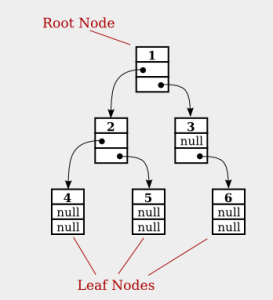
| Barnes-Hut [checklist] |
Simulate the motion of N bodies, mutually affected by gravitational forces when N is large. | quad-tree, analysis of algorithms, data abstraction | 8 |
| Particle Collision Simulation | Simulate the motion of N colliding particles according to the laws of elastic collision. | priority queue, event-driven simulation | 7 |
| Atomic Nature of Matter [checklist] |
Estimate Avogadro's number using video microscopy of Brownian motion. | depth-first search, image processing, data abstraction, data analysis | 8 |
| Root Finding [checklist] |
Compute square roots using Newton's method. | loops, numerical computation | 2 |
| Cracking the Genetic Codes [checklist] |
Find the genetic encoding of amino acids, given a protein and a genetic sequence known to contain that protein. | strings, file input | 5 |
| RECREATION | |||
|---|---|---|---|
| Mozart Waltz Generator | Create a two-part waltz using Mozart's dice game. | arrays | 3 |
| Rogue [checklist] |
Given a dungeon of rooms and corridors, and two players (monster and rogue) that alternate moves, devise a strategy for the monster to intercept the rogue, and devise a strategy for the rogue to evade the monster. | graph, breath first search, depth first search, bridges | 8 |
| 8 Slider Puzzle [checklist] |
Solve Sam Loyd's 8 slider puzzle using AI. | priority queue, A* algorithm | 5 |
| GRAPHICS AND IMAGE PROCESSING | |||
|---|---|---|---|
| Mandelbrot Set [checklist] |
Plot the Mandelbrot set. | functions, arrays, graphics | 3 |
| H-tree [checklist] |
Draw recursive patterns. | recursion, graphics | 3 |
| Sierpinski Triangle [checklist] |
Draw recursive patterns. | recursion, graphics | 3 |
| Collinear Points [checklist] |
Given a set of Euclidean points, determine any groups of 4 or more that are collinear. | polar sorting, analysis of algorithms | 4 |
| Smallest Enclosing Circle [checklist] |
Given a set of Euclidean points, determine the smallest enclosing circle. | computational geometry, randomized algorithm | 8 |
| Planar Point Location [checklist] |
Read in a set of lines and determine whether two query points are separated by any line. | computational geometry, binary tree | 6 |
| COMBINATORIAL OPTIMIZATION | |||
|---|---|---|---|
| Small World Phenomenon | Use the Internet Movie Database to compute Kevin Bacon numbers. | graph, breadth-first search, symbol table | 7 |
| Map Routing | Read in a map of the US and repeatedly compute shortest paths between pairs of points. | graph, Dijkstra's algorithm, priority queue, A* algorithm. | 7 |
| Bin Packing | Allocate sound files of varying sizes to disks to minimize the number of disks. | priority queue, binary search tree, approximation algorithm | 5 |
| Traveling Salesperson Problem | Find the shortest route connecting 13,509 US cities. | linked list, heuristics | 5 |
| Open Pit Mining | Given an array of positive and negative expected returns, find a contiguous block that maximizes the expected profit. | divide-and-conquer, analysis of algorithms | 5 |
| Baseball Elimination | Given the standings of a sports league, determine which teams are mathematically eliminated. | reduction, max flow, min cut | 3 |
| Assignment Problem | Solve the assignment problem by reducing it to min cost flow. | reduction, min cost flow | 3 |
| Password Cracking | Crack a subset-sum password authentication scheme. | hashing, space-time tradeoff | |
| TEXT PROCESSING | |||
|---|---|---|---|
| Natural Language Modeling | Create a Markov model of an input text and use it to automatically generate stylized pseudo-random text. | suffix sorting or hashing | 6 |
| Natural Language Modeling | Create a Markov model of an input text and use it to automatically generate stylized pseudo-random text. | Markov chains, graph | 4 |
| Markovian Candidate [checklist] |
Create a Markov model of an input text to perform speech attribution. | artificial intelligence, symbol table | 6 |
| Word Searching | Search for words horizontally, vertically and diagonally in a 2D character array | tries | 7 |
| Redundancy Detector | Find the longest repeated sequence in a given text. | suffix sorting, strings | 4 |
| Text Indexing | Build an inverted index of a text corpus and find the position of query strings in the text. | suffix sorting or binary search tree | 4 |
| COMMUNICATION | |||
|---|---|---|---|
| Linear Feedback Shift Register | Encrypt images using a linear feedback shift register. | objects, encryption | 4 |
| Pictures from Space | Detect and fix data errors in transmission using a Hadamard code. | 2D arrays, error-correcting codes | 3 |
| Prefix Free Codes | Decode a message compressed using Huffman codes. | binary trees, data compression | 4 |
| Burrows-Wheeler | Implement a novel text compression scheme that out-compresses PKZIP. | suffix sorting, arrays, data compression | 7 |
| RSA Cryptosystem | Implement the RSA cryptosystem. | big integers, repeated squaring, analysis of algorithms | 8 |
| DISCRETE MATH | |||
|---|---|---|---|
| Linked List Sort | Shellsort a linked list. | linked list, shellsort | 4 |
| Batcher Sort | Implement Batcher's even-odd mergesort. | divide-and-conquer, parallel sorting hardware | 6 |
| Rational Arithmetic | Implement a Rational number data type. | struct, data abstraction, Euclid's algorithm | 3 |
| Factoring | Factor large integers using Pollard's rho method. | big integers, Euclid's algorithm | 5 |
| Deques and Randomized Queues | Create deque and randomized queue ADTs. | abstract data types, generics | 5 |
| Linear Congruential Random Number Generator | Find the cycle length of a pseudo-random number generator using Floyd's algorithm. | loops, mod | 2 |
| Stock Market | Predict the performance of a stock using Dilbert's rule. | loops | 2 |
| Subset Sum | Partition the square roots of 1 to 100 into two subsets so that their sum is as close as possible to each other. | various | 6 |
| Loops and Conditionals | Binary logarithm, checkerboard pattern, random walk, Gaussian distribution. | loops and conditionals | 1 |
Here are some Nifty Assignments created by instructors at other universities. They are more oriented towards recreational applications, but are fun and creative.
Copyright © 2000–2019 Robert Sedgewick and Kevin Wayne. All rights reserved.
Molecular Dynamics Simulation of Hard Spheres
COS 226 Programming Assignment
Molecular Dynamics Simulation of Hard Spheres
Simulate the motion of N colliding particles according to the laws of elastic collision using event-driven simulation. Such simulations are widely used in molecular dynamics (MD) to understand and predict properties of physical systems at the particle level. This includes the motion of molecules in a gas, the dynamics of chemical reactions, atomic diffusion, sphere packing, the stability of the rings around Saturn, the phase transitions of cerium and cesium, one-dimensional self-gravitating systems, and front propagation. The same techniques apply to other domains that involve physical modeling of particle systems including computer graphics, computer games, and robotics.
Hard sphere model. The hard sphere model (billiard ball model) is an idealized model of the motion of atoms or molecules in a container. In this assignment, we will focus on the two-dimensional version called the hard disc model. The salient properties of this model are listed below.
- N particles in motion, confined in the unit box.
- Particle i has known position (rxi, ryi), velocity (vxi, vyi), mass mi, and radius σi.
- Particles interact via elastic collisions with each other and with the reflecting boundary.
- No other forces are exerted. Thus, particles travel in straight lines at constant speed between collisions.
This simple model plays a central role in statistical mechanics, a field which relates macroscopic observables (e.g., temperature, pressure, diffusion constant) to microscopic dynamics (motion of individual atoms and molecules). Maxwell and Boltzmann used the model to derive the distribution of speeds of interacting molecules as a function of temperature; Einstein used it to explain the Brownian motion of pollen grains immersed in water.
Simulation. There are two natural approaches to simulating the system of particles.
- Time-driven simulation. Discretize time into quanta of size dt. Update the position of each particle after every dt units of time and check for overlaps. If there is an overlap, roll back the clock to the time of the collision, update the velocities of the colliding particles, and continue the simulation. This approach is simple, but it suffers from two significant drawbacks. First, we must perform N2 overlap checks per time quantum. Second, we may miss collisions if dt is too large and colliding particles fail to overlap when we are looking. To ensure a reasonably accurate simulation, we must choose dt to be very small, and this slows down the simulation.
- Event-driven simulation. With event-driven simulation we focus on those times at which interesting events occur. In the hard disc model, all particles travel in straight line trajectories at constant speeds between collisions. Thus, our main challenge is to determine the ordered sequence of particle collisions. We address this challenge by maintaining a priority queue of future events, ordered by time. At any given time, the priority queue contains all future collisions that would occur, assuming each particle moves in a straight line trajectory forever. As particles collide and change direction, some of the events scheduled on the priority queue become "stale" or "invalidated", and no longer correspond to physical collisions. We can adopt a lazy strategy, leaving such invalidated collision on the priority queue, waiting to identify and discard them as they are deleted. The main event-driven simulation loop works as follows:
- Delete the impending event, i.e., the one with the minimum priority t.
- If the event corresponds to an invalidated collision, discard it. The event is invalid if one of the particles has participated in a collision since the event was inserted onto the priority queue.
- If the event corresponds to a physical collision between particles i and j:
- Advance all particles to time t along a straight line trajectory.
- Update the velocities of the two colliding particles i and j according to the laws of elastic collision.
- Determine all future collisions that would occur involving either i or j, assuming all particles move in straight line trajectories from time t onwards. Insert these events onto the priority queue.
- If the event corresponds to a physical collision between particles i and a wall, do the analogous thing for particle i.
This event-driven approach results in a more robust, accurate, and efficient simulation than the time-driven one.
Collision prediction. In this section we present the formulas that specify if and when a particle will collide with the boundary or with another particle, assuming all particles travel in straight-line trajectories.
- Collision between particle and a wall. Given the position (rx, ry), velocity (vx, vy), and radius σ of a particle at time t, we wish to determine if and when it will collide with a vertical or horizontal wall.
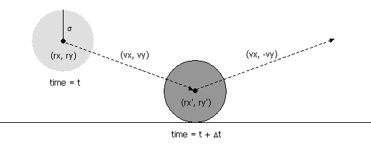
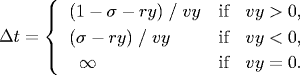
An analogous equation predicts the time of collision with a vertical wall.
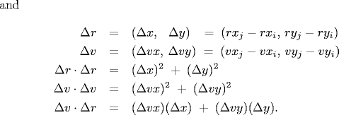
- Collision between two particles. Given the positions and velocities of two particles i and j at time t, we wish to determine if and when they will collide with each other.
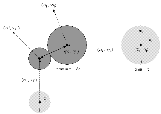
σ2 = (rxi' - rxj' )2 + (ryi' - ryj' )2
During the time prior to the collision, the particles move in straight-line trajectories. Thus,
rxi' = rxi + Δt vxi, ryi' = ryi + Δt vyi
rxj' = rxj + Δt vxj, ryj' = ryj + Δt vyjSubstituting these four equations into the previous one, solving the resulting quadratic equation for Δt, selecting the physically relevant root, and simplifying, we obtain an expression for Δt in terms of the known positions, velocities, and radii.
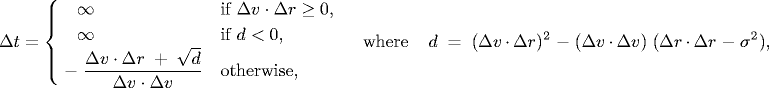
If either Δv ⋅ Δr ≥ 0 or d < 0, then the quadratic equation has no solution for Δt > 0; otherwise we are guaranteed that Δt ≥ 0.
Collision resolution. In this section we present the physical formulas that specify the behavior of a particle after an elastic collision with a reflecting boundary or with another particle. For simplicity, we ignore multi-particle collisions. There are three equations governing the elastic collision between a pair of hard discs: (i) conservation of linear momentum, (ii) conservation of kinetic energy, and (iii) upon collision, the normal force acts perpendicular to the surface at the collision point. Physics-ly inclined students are encouraged to derive the equations from first principles; the rest of you may keep reading.
- Between particle and wall. If a particle with velocity (vx, vy) collides with a wall perpendicular to x-axis, then the new velocity is (-vx, vy); if it collides with a wall perpendicular to the y-axis, then the new velocity is (vx, -vy).
- Between two particles. When two hard discs collide, the normal force acts along the line connecting their centers (assuming no friction or spin). The impulse (Jx, Jy) due to the normal force in the x and y directions of a perfectly elastic collision at the moment of contact is:

and where mi and mj are the masses of particles i and j, and σ, Δx, Δy and Δ v ⋅ Δr are defined as above. Once we know the impulse, we can apply Newton's second law (in momentum form) to compute the velocities immediately after the collision.
vxi' = vxi + Jx / mi, vxj' = vxj - Jx / mj
vyi' = vyi + Jy / mi, vyj' = vyj - Jy / mj
Data format. Use the following data format. The first line contains the number of particles N. Each of the remaining N lines consists of 6 real numbers (position, velocity, mass, and radius) followed by three integers (red, green, and blue values of color). You may assume that all of the position coordinates are between 0 and 1, and the color values are between 0 and 255. Also, you may assume that none of the particles intersect each other or the walls.
N
rx ry vx vy mass radius r g b
rx ry vx vy mass radius r g b
rx ry vx vy mass radius r g b
rx ry vx vy mass radius r g b
Your task. Write a program MDSimulation.java that reads in a set of particles from standard input and animates their motion according to the laws of elastic collisions and event-driven simulation.
Perhaps everything below is just for the checklist??
Particle collision simulation in Java. There are a number of ways to design a particle collision simulation program using the physics formulas above. We will describe one such approach, but you are free to substitute your own ideas instead. Our approach involves the following data types: MinPQ, Particle, CollisionSystem, and Event.
- Priority queue. A standard priority queue where we can check if the priority queue is empty; insert an arbitrary element; and delete the minimum element.
- Particle data type. Create a data type to represent particles moving in the unit box. Include private instance variables for the position (in the x and y directions), velocity (in the x and y directions), mass, and radius. It should also have the following instance methods
- public Particle(...): constructor.
- public double collidesX(): return the duration of time until the invoking particle collides with a vertical wall, assuming it follows a straight-line trajectory. If the particle never collides with a vertical wall, return a negative number (or +infinity = DOUBLE_MAX or NaN???)
- public double collidesY(): return the duration of time until the invoking particle collides with a horizontal wall, assuming it follows a straight-line trajectory. If the particle never collides with a horizontal wall, return a negative number.
- public double collides(Particle b): return the duration of time until the invoking particle collides with particle b, assuming both follow straight-line trajectories. If the two particles never collide, return a negative value.
- public void bounceX(): update the invoking particle to simulate it bouncing off a vertical wall.
- public void bounceY(): update the invoking particle to simulate it bouncing off a horizontal wall.
- public void bounce(Particle b): update both particles to simulate them bouncing off each other.
- public int getCollisionCount(): return the total number of collisions involving this particle.
- Event data type. Create a data type to represent collision events. There are four different types of events: a collision with a vertical wall, a collision with a horizontal wall, a collision between two particles, and a redraw event. This would be a fine opportunity to experiment with OOP and polymorphism. We propose the following simpler (but somewhat less elegant approach).
- public Event(double t, Particle a, Particle b): Create a new event representing a collision between particles a and b at time t. If neither a nor b is null, then it represents a pairwise collision between a and b; if both a and b are null, it represents a redraw event; if only b is null, it represents a collision between a and a vertical wall; if only a is null, it represents a collision between b and a horizontal wall.
- public double getTime(): return the time associated with the event.
- public Particle getParticle1(): return the first particle, possibly null.
- public Particle getParticle2(): return the second particle, possibly null.
- public int compareTo(Object x): compare the time associated with this event and x. Return a positive number (greater), negative number (less), or zero (equal) accordingly.
- public boolean wasSuperveningEvent(): return true if the event has been invalidated since creation, and false if the event has been invalidated.
In order to implement wasSuperveningEvent, the event data type should store the collision counts of two particles at the time the event was created. The event corresponds to a physical collision if the current collision counts of the particles are the same as when the event was created.
- Particle collision system. The main program containing the event-driven simulation. Follow the event-driven simulation loop described above, but also consider collisions with the four walls and redraw events.
Data sets. Some possibilities that we'll supply.
- One particle in motion.
- Two particles in head on collision.
- Two particles, one at rest, colliding at an angle.
- Some good examples for testing and debugging.
- One red particle in motion, N blue particles at rest.
- N particles on a lattice with random initial directions (but same speed) so that the total kinetic energy is consistent with some fixed temperature T, and total linear momentum = 0. Have a different data set for different values of T.
- Diffusion I: assign N very tiny particles of the same size near the center of the container with random velocities.
- Diffusion II: N blue particles on left, N green particles on right assigned velocities so that they are thermalized (e.g., leave partition between them and save positions and velocities after a while). Watch them mix. Calculate average diffusion rate?
- N big particles so there isn't much room to move without hitting something.
- Einstein's explanation of Brownian motion: 1 big red particle in the center, N smaller blue particles.
Things you could compute.
- Brownian motion. In 1827, the botanist Robert Brown observed the motion of wildflower pollen grains immersed in water using a microscope. He observed that the pollen grains were in a random motion, following what would become known as Brownian motion. This phenomenon was discussed, but no convincing explanation was provided until Einstein provided a mathematical one in 1905. Einstein's explanation: the motion of the pollen grain particles was caused by millions of tiny molecules colliding with the larger particles. He gave detailed formulas describing the behavior of tiny particles suspended in a liquid at a given temperature. Einstein's explanation was intended to help justify the existence of atoms and molecules and could be used to estimate the size of the molecules. Einstein's theory of Brownian motion enables engineers to compute the diffusion constants of alloys by observing the motion of individual particles. Here's a flash demo of Einstein's explanation of Brownian motion from here.
- Free path and free time. Free path = distance a particle travels between collisions. Plot histogram. Mean free path = average free path length over all particles. As temperature increases, mean free path increases (holding pressure constant). Compute free time length = time elapsed before a particle collides with another particle or wall.
- Collision frequency. Number of collisions per second.
- Root mean-square velocity. Root mean-square velocity / mean free path = collision frequency. Root mean square velocity = sqrt(3RT/M) where molar gas constant R = 8.314 J / mol K, T = temperature (e.g., 298.15 K), M = molecular mass (e.g., 0.0319998 kg for oxygen).
- Maxwell-Boltzmann distribution. Distribution of velocity of particles in hard sphere model obey Maxwell-Boltzmann distribution (assuming system has thermalized and particles are sufficiently heavy that we can discount quantum-mechanical effects). Distribution shape depends on temperature. Velocity of each component has distribution proportional to exp(-mv_x^2 / 2kT). Magnitude of velocity in d dimensions has distribution proportional to v^(d-1) exp(-mv^2 / 2kT). Used in statistical mechanics because it is unwieldy to simulate on the order of 10^23 particles. Reason: velocity in x, y, and z directions are normal (if all particles have same mass and radius). In 2d, Rayleigh instead of Maxwell-Boltzmann.
- Pressure. Main thermodynamic property of interest = mean pressure. Pressure = force per unit area exerted against container by colliding molecules. In 2d, pressure = average force per unit length on the wall of the container.
- Temperature. Plot temperature over time (should be constant) = 1/N sum(mv^2) / (d k), where d = dimension = 2, k = Boltzmann's constant.
- Diffusion. Molecules travel very quickly (faster than a speeding jet) but diffuse slowly because they collide with other molecules, thereby changing their direction. Two vessels connected by a pipe containing two different types of particles. Measure fraction of particles of each type in each vessel as a function of time.
- Time reversibility. Change all velocities and run system backwards. Neglecting roundoff error, the system will return to its original state!
- Maxwell's demon. Maxwell's demon is a thought experiment conjured up by James Clerk Maxwell in 1871 to contradict the second law of thermodynamics. Vertical wall in middle with molecule size trap door, N particles on left half and N on right half, particle can only go through trap door if demon lets it through. Demon lets through faster than average particles from left to right, and slower than average particles from right to left. Can use redistribution of energy to run a heat engine by allowing heat to flow from left to right. (Doesn't violate law because demon must interact with the physical world to observe the molecules. Demon must store information about which side of the trap door the molecule is on. Demon eventually runs out of storage space and must begin erasing previous accumulated information to make room for new information. This erasing of information increases the entropy, requiring kT ln 2 units of work.)
Cell method. Useful optimization: divide region into rectangular cells. Ensure that particles can only collide with particles in one of 9 adjacent cells in any time quantum. Reduces number of binary collision events that must be calculated. Downside: must monitor particles as they move from cell to cell.
Extra credit. Handle multi-particle collisions. Such collisions are important when simulating the break in a game of billiards.
This assignment was developed by Ben Tsou and Kevin Wayne.Copyright © 2004.
Last modified on January 31, 2009.
Copyright © 2000–2019 Robert Sedgewick and Kevin Wayne. All rights reserved.
Monte Carlo Simulation
https://introcs.cs.princeton.edu/java/98simulation/
This section under major construction.
In 1953 Enrico Fermi, John Pasta, and Stanslaw Ulam created the first "computer experiment" to study a vibrarting atomic lattice. Nonlinear system couldn't be analyzed by classical mathematics.
Simulation = analytic method that imitates a physical system. Monte Carlo simulation = use randomly generated values for uncertain variables. Named after famous casino in Monaco. At essentially each step in the evolution of the calculation, Repeat several times to generate range of possible scenarios, and average results. Widely applicable brute force solution. Computationally intensive, so use when other techniques fail. Typically, accuracy is proportional to square root of number of repetitions. Such techniques are widely applied in various domains including: designing nuclear reactors, predicting the evolution of stars, forecasting the stock market, etc.
Generating random numbers. The math library function Math.random generate a pseudo-random number greater than or equal to 0.0 and less than 1.0. If you want to generate random integers or booleans, the best way is to use the library Random. Program RandomDemo.java illustrates how to use it.
Note that you should only create a new Random object once per program. You will not get more "random" results by creating more than one. For debugging, you may wish to produce the same sequence of pseudo-random number each time your program executes. To do this, invoke the constructor with a long argument.
The pseudo-random number generator will use 1234567 as the seed. Use SecureRandom for cryptographically secure pseudo-random numbers, e.g., for cryptography or slot machines.
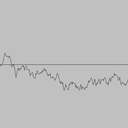
Linear congruential random number generator. With integer types we must be cognizant of overflow. Consider a * b (mod m) as an example (either in context of a^b (mod m) or linear congruential random number generator: Given constants a, c, m, and a seed x[0], iterate: x = (a * x + c) mod m. Park and Miller suggest a = 16807, m = 2147483647, c = 0 for 32-bit signed integers. To avoid overflow, use Schrage's method.
Exercise: compute cycle length.
Library of probability functions. OR-Objects contains many classic probability distributions and random number generators, including Normal, F, Chi Square, Gamma, Binomial, Poisson. You can download the jar file here. Program ProbDemo.java illustrates how to use it. It generate one random value from the gamma distribution and 5 from the binomial distribution. Note that the method is called getRandomScaler and not getRandomScalar.
Queuing models. M/M/1, etc. A manufacturing facility has M identical machines. Each machine fails after a time that is exponentially distributed with mean 1 / μ. A single repair person is responsible for maintaining all the machines, and the time to fix a machine is exponentially distributed with mean 1 / λ. Simulate the fraction of time in which no machines are operational.
Diffusion-limited aggregation.
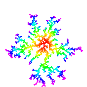
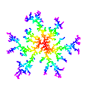
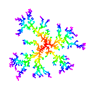
Diffuse = undergo random walk. The physical process diffusion-limited aggregation (DLA) models the formation of an aggregate on a surface, including lichen growth, the generation of polymers out of solutions, carbon deposits on the walls of a cylinder of a Diesel engine, path of electric discharge, and urban settlement.
The modeled aggregate forms when particles are released one at a time into a volume of space and, influenced by random thermal motion, they diffuse throughout the volume. There is a finite probability that the short-range attraction between particles will influence the motion. Two particles which come into contact with each other will stick together and form a larger unit. The probability of sticking increases as clusters of occupied sites form in the aggregate, stimulating further growth. Simulate this process in 2D using Monte Carlo methods: Create a 2D grid and introduce particles to the lattice through a launching zone one at a time. After a particle is launched, it wanders throughout with a random walk until it either sticks to the aggregate or wanders off the lattice into the kill zone. If a wandering particle enters an empty site next to an occupied site, then the particle's current location automatically becomes part of the aggregate. Otherwise, the random walk continues. Repeat this process until the aggregate contains some pre-determined number of particles. Reference: Wong, Samuel, Computational Methods in Physics and Engineering, 1992.
Program DLA.java simulates the growth of a DLA with the following properties. It uses the helper data type Picture.java. Set the initial aggregate to be the bottom row of the N-by-N lattice. Launch the particles from a random cell in top row. Assume that the particle goes up with probability 0.15, down with probability 0.35, and left or right with probability 1/4 each. Continue until the particles stick to a neighboring cell (above, below, left, right, or one of the four diagonals) or leaves the N-by-N lattice. The preferred downward direction is analogous to the effect of a temperature gradient on Brownian motion, or like how when a crystal is formed, the bottom of the aggregate is cooled more than the top; or like the influence of a gravitational force. For effect, we color the particles in the order they are released according to the rainbow from red to violet. Below are three simulations with N = 176; here is an image with N = 600.
 |
 |
 |
Brownian motion. Brownian motion is a random process used to model a wide variety of physical phenomenon including the dispersion of ink flowing in water, and the behavior of atomic particles predicted by quantum physics. (more applications). Fundamental random process in the universe. It is the limit of a discrete random walk and the stochastic analog of the Gaussian distribution. It is now widely used in computational finance, economics, queuing theory, engineering, robotics, medical imaging, biology, and flexible manufacturing systems. First studied by a Scottish botanist Robert Brown in 1828 and analyzed mathematically by Albert Einstein in 1905. Jean-Baptiste Perrin performed experiments to confirm Einstein's predictions and won a Nobel Prize for his work. An applet to illustrate physical process that may govern cause of Brownian motion.
Simulating a Brownian motion. Since Brownian motion is a continuous and stochastic process, we can only hope to plot one path on a finite interval, sampled at a finite number of points. We can interpolate linearly between these points (i.e., connect the dots). For simplicitly, we'll assume the interval is from 0 to 1 and the sample points t0, t1, ..., tN are equally spaced in this interval. To simulate a standard Brownian motion, repeatedly generate independent Gaussian random variables with mean 0 and standard deviation sqrt(1/N). The value of the Brownian motion at time i is the sum of the first i increments.
 |
 |
 |
Black-Scholes formula. Move to here?
Ising model. The motions of electrons around a nucleus produce a magnetic field associated with the atom. These atomic magnets act much like conventional magnets. Typically, the magnets point in random directions, and all of the forces cancel out leaving no overall magnetic field in a macroscopic clump of matter. However, in some materials (e.g., iron), the magnets can line up producing a measurable magnetic field. A major achievement of 19th century physics was to describe and understand the equations governing atomic magnets. The probability that state S occurs is given by the Boltzmann probability density function P(S) = e-E(S)/kT / Z, where Z is the normalizing constant (partition function) sum e-E(A)/kT over all states A, k is Boltzmann's constant, T is the absolute temperature (in degrees Kelvin), and E(S) is the energy of the system in state S.
Ising model proposed to describe magnetism in crystalline materials. Also models other naturally occurring phenomena including: freezing and evaporation of liquids, protein folding, and behavior of glassy substances.
Ising model. The Boltzmann probability function is an elegant model of magnetism. However, it is not practical to apply it for calculating the magnetic properties of a real iron magnet because any macroscopic chunk of iron contains an enormous number atoms and they interact in complicated ways. The Ising model is a simplified model for magnets that captures many of their important properties, including phase transitions at a critical temperature. (Above this temperature, no macroscopic magnetism, below it, systems exhibits magnetism. For example, iron loses its magnetization around 770 degrees Celsius. Remarkable thing is that transition is sudden.) reference
First introduced by Lenz and Ising in the 1920s. In the Ising model, the iron magnet is divided into an N-by-N grid of cells. (Vertex = atom in crystal, edge = bond between adjacent atoms.) Each cell contains an abstract entity known as spin. The spin si of cell i is in one of two states: pointing up (+1) or pointing down (-1). The interactions between cells is limited to nearest neighbors. The total magnetism of the system M = sum of si. The total energy of the system E = sum of - J si sj, where the sum is taken over all nearest neighbors i and j. The constant J measures the strength of the spin-spin interactions (in units of energy, say ergs). [The model can be extended to allow interaction with an external magnetic field, in which case we add the term -B sum of sk over all sites k.] If J > 0, the energy is minimized when the spins are aligned (both +1 or both -1) - this models ferromagnetism. if J < 0, the energy is minimized when the spins are oppositely aligned - this models antiferromagnetism.
Given this model, a classic problem in statistical mechanics is to compute the expected magenetism. A state is the specification of the spin for each of the N^2 lattice cells. The expected magnetism of the system E[M] = sum of M(S) P(S) over all states S, where M(S) is the magnetism of state S, and P(S) is the probability of state S occurring according to the Boltzmann probability function. Unfortunately, this equation is not amenable to a direct computational because the number of states S is 2N*N for an N-by-N lattice. Straightforward Monte Carlo integration won't work because random points will not contribute much to sum. Need selective sampling, ideally sample points proportional to e-E/kT. (In 1925, Ising solved the problem in one dimension - no phase transition. In a 1944 tour de force, Onsager solved the 2D Ising problem exactly. His solution showed that it has a phase transition. Not likely to be solved in 3D - see intractability section.)
Metropolis algorithm. Widespread usage of Monte Carlo methods began with Metropolis algorithm for calculation of rigid-sphere system. Published in 1953 after dinner conversation between Metropolis, Rosenbluth, Rosenbluth, Teller, and Teller. Widely used to study equilibrium properties of a system of atoms. Sample using Markov chain using Metropolis' rule: transition from A to B with probability 1 if Δ E <= 0, and with probability e-ΔE/kT if Δ E > 0. When applied to the Ising model, this Markov chain is ergodic (similar to Google PageRank requirement) so the theory underlying the Metropolis algorithm applies. Converges to stationary distribution.
Program Cell.java, State.java, and Metropolis.java implements the Metropolis algorithm for a 2D lattice. Ising.java is a procedural programming version. "Doing physics by tossing dice." Simulate complicated physical system by a sequence of simple random steps.
Measuring physical quantities. Measure magnetism, energy, specific heat when system has thermalized (the system has reached a thermal equilibrium with its surrounding environment at a common temperature T). Compute the average energy and the average magenetization over time. Also interesting to compute the variance of the energy or specific heat <c> = <E2> - <E>2, and the variance of the magnetization or susceptibility <Χ> = <M2> - <M>2. Determining when system has thermalized is a challenging problem - in practice, many scientists use ad hoc methods.
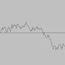
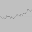
Phase transition. Phase transition occurs when temperature Tc is 2 / ln(1 + sqrt(2)) = 2.26918). Tc is known as the Curie temperature. Plot magnetization M (average of all spins) vs. temperature (kT = 1 to 4). Discontinuity of slope is signature of second order phase transition. Slope approaches infinity. Plot energy (average of all spin-spin interactions) vs. temperature (kT = 1 to 4). Smooth curve through phase transition. Compare against exact solution. Critical temperature for which algorithm dramatically slows down. Below are the 5000th sample trajectory for J/kT = 0.4 (hot / disorder) and 0.47 (cold / order). The system becomes magnetic as temperature decreases; moreover, as temperature decreases the probability that neighboring sites have the same spin increasing (more clumping).
Experiments.
- Start will above critical temperature. State converges to nearly uniform regardless of initial state (all up, all down, random) and fluctuates rapidly. Zero magnetization.
- Start well below critical temperature. Start all spins with equal value (all up or all down). A few small clusters of opposite spin form.
- Start well below critical temperature. Start with random spins. Large clusters of each spin form; eventually simulation makes up its mind. Equally likely to have large clusters in up or down spin.
- Start close to critical temperature. Large clusters form, but fluctuate very slowly.
 |
 |
Exact solution for Ising model known for 1D and 2D; NP-hard for 3d and nonplanar graphs.
Models phase changes in binary alloys and spin glasses. Also models neural networks, flocking birds, and beating heart cells. Over 10,000+ papers published using the Ising model.
Q + A
Exercises
- Print a random word. Read in a list of words (of unknown length) from standard input, and print out one of the N words uniformly at random. Do not store the word list. Instead, use Knuth's method: when reading in the ith word, select it with probability 1/i to be the new champion. Print out the word that survives after reading in all of the data.
- Random subset of a linked list. Given an array of N elements and an integer k ≤ N, construct a new array containing a random subset of k elements. Hint: traverse the array, either accepting each element with probability a/b, where a is the number of elements left to select, and b is the number of elements remaining.
Creative Exercises
- Random number generation. Can the following for computing a pseudo-random integer between 0 and N-1 fail? Math.random is guaranteed to return a floating point number greater than or equal to 0.0 and strictly less than 1.0.
double x = Math.random();
int r = (int) (x * N);
That is, can you find a real number x and an integer N for which r equals N?
Solution: No, it can't happen in IEEE floating point arithmetic. The roundoff error will not cause the result to be N, even if Math.random returns 0.9999999999.... However, this method does not produce integers uniformly at random because floating point numbers are not evenly distributed. Also, it involves casting and multiplying, which are excessive.
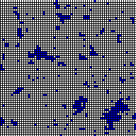
- Random number test. Write a program to plot the outcome of a boolean pseudo-random number generator. For simplicity, use (Math.random() < 0.5) and plot in a 128-by-128 grid like the following pseudorandom applet. Perhaps use LFSR or Random.nextLong() % 2.
- Sampling from a discrete probability distribution. Suppose that there are N events and event i occurs with probability pi, where p0 + p1 + ... + pN-1 = 1. Write a program Sample.java that prints out 1,000 sample events according to the probability distribution. Hint: choose a random number r between 0 and 1 and iterate from i = 0 to N-1 until p0 + p1 + ... + pi > r. (Be careful about floating point precision.)
- Sampling from a discrete probability distribution. Improve the algorithm from the previous problem so that it takes time proportional to log N to generate a new sample. Hint: binary search on the cumulative sums. Note: see this paper for a very clever alternative that generates random samples in a constant amount of time. Discrete.java is a Java version of Warren D. Smith's WDSsampler.c program.
- Sampling from a discrete probability distribution. Repeat the previous question but make it dynamic. That is, after each sample, the probabilities of some events might change, or there may be new events. Used in n-fold way algorithm, which is method of choice for kinetic Monte Carlo methods where one wants to simulate the kinetic evolution process. Typical application: simulating gas reacting with surface of a substrate where chemical reaction occur at different rates. Hint: use a binary search tree.
- Zipf distribution. Use the result of the previous exercise(s) to sample from the Zipfian distribution with parameter s and N. The distribution can take on integer values from 1 to N, and takes on value k with probability 1/k^s / sum_(i = 1 to N) 1/i^s. Example: words in Shakespeare's play Hamlet with s approximately equal to 1.
- Simulating a Markov chain. Write a program MarkovChain.java that simulates a Markov chain. Hint: you will need to sample from a discrete distribution.
- DLA with non-unity sticking probability Modify DLA.java so that the initial aggregate consists of several randomly spaced cells along the bottom of the lattice. This simulates string-like bacterial growth.
- DLA with non-unity sticking probability Modify DLA.java to allow a sticking probability less than one. That is, if a particle has a neighbor, then it sticks with probability p < 1.0; otherwise, it moves at random to a neighboring cell which is unoccupied. This results in a gives more clustered structure, simulating higher bond affinity between atoms.
- Symmetric DLA. Initialize the aggregate to be a single particle in the center of the lattice. Launch particles uniformly from a circle centered at the initial particle. Increase the size of the launch circle as the size of the aggregate increases. Name your program SymmetricDLA.java. This simulates the growth of an aggregate where the particles wander in randomly from infinity. Here are some tricks for speeding up the process.
- Variable sticking probability. A wandering particle which enters an empty site next to an occupied site is assigned a random number, indicating a potential direction in which the particle can move (up, down, left or right). If an occupied site exists on the new site indicated by the random number, then the particle sticks to the aggregate by occupying its current lattice site. If not, it moves to that site and the random walk continues. This simulates snowflake growth.
- Random walk solution of Laplace's equation. Numerically solve Laplace's equation to determine the electric potential given the positions of the charges on the boundary. Laplace's equation says that the gradient of the potential is the sum of the second partial derivatives with respect to x and y. See Gould and Tobochnik, 10.2. Your goal is to find the function V(x, y) that satisfies Laplace's equation at specified boundary conditions. Assume the charge-free region is a square and that the potential is 10 along the vertical boundaries and 5 along the horizontal ones. To solve Laplace's equation, divide the square up into an N-by-N grid of points. The potential V(x, y) of cell (x, y) is the average of the potentials at the four neighboring cells. To estimate V(x, y), simulate 1 million random walkers starting at cell (x, y) and continuing until they reach the boundary. An estimate of V(x, y) is the average potential at the 1 million boundary cells reached. Write a program Laplace.java that takes three command line parameters N, x, and y and estimates V(x, y) over an N-by-N grid of cells where the potential at column 0 and N is 10 and the potential at row 0 and N is 5.Remark: although the boundary value problem above can be solved analytically, numerical simulations like the one above are useful when the region has a more complicated shape or needs to be repeated for different boundary conditions.
simulated annealing
- Simulating a geometric random variable. If some event occurs with probability p, a geometric random variable with parameter p models the number N of independent trials needed between occurrence of the event. To generate a variable with the geometric distribution, use the following formula
N = ceil(ln U / ln (1 - p))
where U is a variable with the uniform distribution. Use the Math library methods Math.ceil, Math.log, and Math.random.
- Simulating an exponential random variable. The exponential distribution is widely used to model the the inter-arrival time between city buses, the time between failure of light bulbs, etc. The probability that an exponential random variable with parameter λ is less than x is F(x) = 1 - eλ x for x >= 0. To generate a random deviate from the distribution, use the inverse function method: output -ln(U) / λ where U is a uniform random number between 0 and 1.
- Poisson distribution. The Poisson distribution is useful in describing the fluctuations in the number of nuclei that decay in any particular small time interval.
public static int poisson(double c) { double t = 0.0; for (int x = 0; true; x++) { t = t - Math.log(Math.random()) / c; // sum exponential deviates if (t > 1.0) return x; } } - Simulating a Pareto random variable. The Pareto distribution is often used to model insurance claims damages, financial option holding times, and Internet traffic activity. The probability that a Pareto random variable with parameter a is less than x is F(x) = 1 - (1 + x)-a for x >= 0. To generate a random deviate from the distribution, use the inverse function method: output (1-U)-1/a - 1, where U is a uniform random number between 0 and 1.
- Simulating a Cauchy random variable. The density function of a Cauchy random variable is f(x) = 1/(Π(1 + x2)). The probability that a Cauchy random variable is less than x is F(x) = 1/Π (Π/2 + arctan(x)). To generate a random deviate from the distribution, use the inverse function method: output tan(Π(U - 1/2)), where U is a uniform random number between 0 and 1.
- Generate random point inside unit disc. Incorrect to choose set r uniformly between 0 and 1, θ uniformly between 0.0 and 2π, and use (x, y) = (r cosθ, r sinθ). If you do this, more points close to center of disc. Instead, set (x, y) = (√r cos&theta, √r sinθ) Alternatively, generate x and y uniformly between -1 and 1 and accept if x2 + y2 ≤ 1. Plot a random sequence of points using both methods and see the bias.
- Flipping bits. As part of a genetic algorithm, suppose you need to flip N bits independently, each with probability p, where p is some very small constant.
- Method 1: loop through N bits, generate a Bernouilli(p) random variable for each one and flip accordingly. Takes time proportional to N.
- Method 2: generate a Geometric(p) random variable X_0 and flip bit X_0; genereate another Geometric(p) random variable an flip bit X_0 + X_1, and so on. Takes time proportional to Np.
- Method 3: the number of bits to flip in Binomial(N, p). Determine how many bits to flip by approximating with a Gaussian(Np, sigma) random variable. Then flip Z bits, taking care not to avoid duplicates. Takes time proportional to Np, but less calls to transcendental functions.
- Random point inside N-dimensional sphere. Write a program InsideSphere.java that takes a command line parameter N and computes a random point inside an N-dimensional sphere with radius 1. Generate N uniform random variables deviates x1, ..., xN and use this point if
(x1)2 + ... + (xN)2 ≤ 1
Otherwise repeat.
- Random point on surface of an N-dimensional sphere. Write a program Sphere.java that takes a command line parameter N and computes a random point on the surface of an N-dimensional sphere with radius 1 using Brown's method. Brown's method is to compute N independent standard normal deviates x1, xN. Then
( x1/r, x2/r, ..., xN/r ), where r = sqrt((x1)2 + ... + (xN)2)
has the desired distribution. Use Exercise xyz from Section 3 to compute standard normal deviates.
- Potts model. The Potts model is a variant of the Ising model where each site has q possible directions. (q = 2 corresponds to Ising) The total energy of the system E = sum of - J sigma(si, sj) over all neighbors. The Kronecker delta function δ(x, y) = 1 if x = y and 0 otherwise.
- 2D Brownian motion. Simulate diffusion of particles in a fluid. Write a data type BrownianParticle.java that represents a particle undergoing a Brownian motion in two dimensions. To do this, simulate two indepedent Brownian motions X(t) and Y(t), and plot (X(t), Y(t)). Create a client program that takes a command line integer N, creates N particles at the origin, and simulates a Brownian motion for the N particles.
- Brownian bridge. A Browian bridge is a constratined Brownian motion, which is required to begin at the origin at time 0, and end at the origin at time T. If X(t) is a Brownian motion then Z(t) = X(t) - (t/T)X(T) is such a process. To plot, store the intermediate values X(t) and plot after you've computed X(T).
- Rainbow. In 1637 Rene Descartes discovered the first scientific explanation for the formation of rainbows. His method involved tracing the internal reflections when a light ray is sent through a a spherical raindrop. Simulate the generation of a rainbow according to model of large number of parallel rays hitting a spherical raindrop. When a light ray hit a raindrop, the ray is reflected and refracted. We use the HSB color format, and choose the hue h at random between 0 (red) and 1 (violet). We use 1.33 + 0.06 * h for the refraction index of hue h. For each ray, we plot a single point of light, according to physical laws of refraction and reflection. Each point of light is then plotted in a random color that the observer will see, either in the primary or secondary rainbow. To perform the simulation, we choose one of the 7 colors uniformly at random. Then, we choose a point (x, y) in the unit circle, centered at (0, 0) and set the impact parameter r = sqrt(x2 + y2). The angle of incidence θi = arcsin(r) and, by Snell's law, the angle of refraction θr = arcsin (r / n), where n is the refraction index. If the light ray is totally reflected only once, it emerges at an angle of θp = 4θr - 2θi, contributing to the primary rainbow. If the light ray is totally reflected a second time, it emerges at an angle of θp = 6θr - 2θi - π, contributing to the secondary rainbow. The intensities Ip and Is of the primary and secondary rays are calculated according to the following transmission and reflection formulas for electromagnetic waves across the boundary of two media.
Ip = 1/2 (s(1-s)2 + p(1-p)2)
Is = 1/2 (s2(1-s)2 + p2(1-p)2)
p = (sin(θi-θr)/sin(θi+θr))2
r = (tan(θi-θr)/tan(θi+θr))2
The color intensities Ip and Is are used to determine the saturation in the HSB color format. Program Rainbow.java simulates this process.

Last modified on January 31, 2009.
Copyright © 2000–2019 Robert Sedgewick and Kevin Wayne. All rights reserved.
The One Programming Language to Rule Them All

There’s a language that sits a layer beneath code, and it yearns to be explored
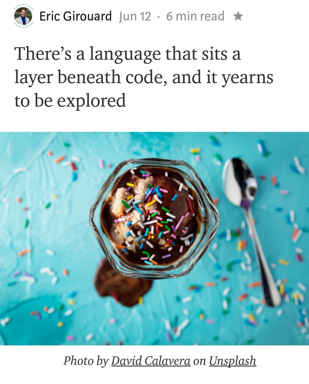
At the time of writing, “which programming language should I learn” yields 517 million search results. Each page will go on about the advantages one language has over the others, and 90% of them will end up recommending Python or JavaScript.
If I may be so bold, I would like to formally disagree with all 517 million of these results and suggest that the first programming language you should learn is logic.
Knowing how to code just doesn’t cut it anymore. The market is so saturated with bootcamp graduates that the “junior software developer” position has been wiped from existence. To succeed today, you need to know how to code and have a logical mindset to boot.
My First Computer Science Lesson
My first exposure to Computer Science was an elective I took in 10th grade. On day one, I was elated to see a wide spread of ice cream and a variety of sundae toppings before me. After we all took our seats, my teacher proclaimed:
“Today, we’re going to be making sundaes. Under one condition: you have to write a list of specific instructions on how to prepare your sundae — then I’ll follow them.”
No problem, I thought, this will be a breeze. In under a minute, I jotted down the perfect set of sundae-making instructions:
Scoop three scoops of black raspberry ice cream into a bowl

Pour two tablespoons of hot fudge into said bowl

Put whipped cream into the bowl

Place sprinkles and a cherry on top of the sundae
Then my teacher — the computer in this lovely metaphor — put on the most accurately sarcastic display I’ve ever seen. She started viciously stabbing the ice cream carton, lid intact, unable to penetrate its tough exterior.
“OK, remove the lid first,” I said, desperate for a treat.
“You failed to provide me with those instructions, so, unfortunately, I failed to make you a sundae, NEXT!”
Fast-forward to attempt #2
Open the black raspberry ice cream by removing the lid

Scoop three scoops of black raspberry ice cream into a bowl

Open the hot fudge and pour two tablespoons into the bowl

Open the whipped cream and add some to the bowl

Place sprinkles and a cherry on top of the sundae
This time I was sure I had it. I even went ahead and ensured each item was opened before adding it to my masterpiece.
She opened the lid, scooped three scoops, and put them into the bowl. At last, my nascent sundae was finally coming into fruition. Then she opened the hot fudge and placed two tablespoons into my bowl. Not two tablespoons of hot fudge, mind you — two actual spoons, and no hot fudge. I failed to be specific enough — again. When all was said and done, I was handed a bowl of ice cream laden with two metal spoons, a solid canister of whipped cream, and about 300 sprinkles.
I think by this point it finally clicked: the computer is a purely logical entity. It has no context and makes no assumptions. It responds to a very specific set of instructions and follows them to a T.
My final set of sundae-making instructions was a verbose, but necessary, disaster:
If they are not already, open each of the following: Black Raspberry Ice Cream, Hot Fudge, Sprinkles, and Whipped Cream

Aquire a bowl from the stack and place it in front of you

Grab the ice cream scoop and, one at a time, scoop three scoops of black raspberry ice cream into the bowl. Place the scoop down when done

Aquire the hot fudge spoon if not already in your possession, then fetch two tablespoons of hot fudge and place them into the bowl, one at a time, and put down the hot fudge when done

Turn the whipped cream upside down, press your finger against the nozzle over the bowl for 3 seconds, and return the bottle to its resting position

Sprinkle approximately 40 sprinkles over the bowl and return the shaker to its upright position when done

Fetch a single cherry from the cherry jar and place it delicately on top of the sundae

Hand the sundae to the student along with a spoon
That last bullet was extremely important because she started eating my sundae without it.
This is the reality of computer programming. Providing intense sets of detailed instructions to a computer. In essence, this is what all programming languages decompose into — instructions.
The Software Development Career Path
Software development is now at a point where it’s too broad to discuss as a single industry, just as “software developer” is too broad a job title. Two developers can be equally marketable while having disjointed skill sets, implying there is more to a career in development than the mere ability to code. There’s an attribute skilled developers have that is universal and separate from programming — logic.
The best developers are experts in critical thinking. This is essential because the majority of software projects are undocumented, splintered disasters. They require a critical thinker to piece information together and fill in the gaps when needed. The developers who lag behind are those who cannot connect the dots.
All this culminates to another bold statement, this time in bold: The fundamentals of computer science are, and will always be, paramount to coding ability.
Popular languages come and go with the tide. Frameworks become deprecated, and companies react to shifting demands by mixing up their tech stack. The one thing that never changes? Fundamentals — that’s literally their definition!
How to Improve Logical Thinking
For those who can’t quite trek a mountain for deep thought, consider these tools to improve your programmatic critical thinking:
Know your run time complexities
Also referred to as Big-O, the runtime complexity of a program can be expressed as the number of steps taken on any instance in relation to the size of the input (n). Keeping perpetual tabs on the runtime of your programs is step one.
Know your data structures
Data structures are at the heart of every complex program. Knowing which structure to use in what scenario is an art of its own. Data structures tie directly into runtime complexities, as picking the wrong structure can send your programs to a grinding halt. Searching an Array for a value is O(n), which means it gets more expensive to use Arrays as the size of your input increases. Hash lookups are O(1), so the lookup time for a Hash key will be constant, regardless of the number of keys in said Hash.
I’ve had candidates argue that an Array has a faster search time than a Hash. This was an immediate signal not to hire them — know your data structures.
Read/watch/listen
Sites like Udemy, Pluralsight, and Codecademy are incredible resources for learning new programming languages. For fundamentals, turn to books on general engineering concepts, best practices, and coding styles. The most highly recommended books for engineers are Design Patterns, Refactoring, Code Complete, Clean Code, and The Pragmatic Programmer, to name a few. Lastly, every engineer should keep a copy of “Introduction to Algorithms” in their desk for safe keeping.
Practice!
You cannot become a master violinist without excessively playing the violin. Sites like HackerRank, CodeWars, CoderByte, TopCoder, and LeetCodehave thousands of challenge problems designed to test your knowledge of data structures and algorithms. The best approach I’ve found to using these sites is to take your own shot at solving the problem, host your solutions on Github, and then look at the top solutions for that problem to see how others approached it. Which brings me to my last point:
View others’ code
The greatest mistake you can make in your software development journey is to go it alone. Software development is a largely crowdsourced effort. We build standards together, make mistakes together, and learn what works over time (by failing a lot). Taking the time to read skilled developers’ code will always pay off. Just make sure it’s good code.
The best advice I can leave you with is to never feel ashamed of what you don’t (yet) know. As I mentioned, this industry is massive, its number of languages extreme, and the content dense. It takes a great deal of time and effort to build an understanding, even more to gain proficiency, and an immense amount more to gain mastery. I’ll let you know when I get there.
Better Programming
Advice for programmers.
Applause from you and 2,671 others

WRITTEN BY
Boston Software Engineer specializing in Hadoop and big-data development. I enjoy writing about that which I’m passionate about.

Princeton University: Programming Assignment Checklist: DNA Sequence Alignment
This assignment allows optional partnering. If you choose to do this, you must follow the pair programming guidelines. Please click the link and review them before you begin. Your partner can be from another precept (but ISC students may only partner with other ISC students). Please note that writing code with a partner without following the pair programming instructions is a violation of the course collaboration policy. All writing of code, comments, analysis and uploading to the dropbox should be done together from start to finish. If you come to office hours alone, you can get advice, but you may not change any code until both partners are together.
What are the main goals of this assignment? You will (i) solve a fundamental problem in computational biology, (ii) learn about the analysis of algorithms, and (iii) learn about a powerful programming paradigm known as dynamic programming.
How do I read in the two input strings from the file? Use StdIn.readString() and redirection as usual.
How do I access the length of a string s? The ith character? Use s.length() and s.charAt(i), respectively. As with arrays, indices start at 0. We'll learn about this notation for manipulating (String) objects in Section 3.1. For this assignment, this is all you'll need to know about objects.
Can I assume that the input characters will always be A, C, G or T? NO! Your program should work equally well for any letter, upper case or lower case.
What's a StringIndexOutOfBoundsException? It's just like an ArrayOutOfBoundsException. It results from invoking s.charAt(i) with an illegal value of i.
How could I get a NullPointerException? Did you forget to allocate memory for opt[][]?
How do I declare and initialize a two dimensional array in Java? Review the end of Section 1.4 in Intro to Programming.
It seems strange to define x[i..M] to be the substring consisting of x[i] through x[M-1] instead of x[i] through x[M]. Is this a typo? It's a little strange, but no, it's not a typo. It's consistent with Java's indexing notation where the left endpoint is inclusive and the right endpoint is exclusive.
Which alignment should I print out if there are two or more optimal ones? Output any one you like.
Should gaps be handled by penalty()? The solution we think is clearest does not call penalty() on gaps, since a gap is not a character. Of course, the alignment output should use the '-'symbol to denote a gap, and the inputs we give you will never contain '-' (only alphanumeric characters are used), so if you find it convenient for penalty() to recognize '-' as a gap, you are permitted to do so.
Where can I learn more about dynamic programming and backtracking? The LCS (longest common subsequence) problem described in booksite section 9.6 is an example of a dynamic programming problem on strings with backtracking. However, it is different from the current problem in many ways, so do not simply mimic the code without understanding what it does. The websheet exercises for this week include several dynamic programming exercises starting from a basic level, including KnapsackBacktrack which is an example of backtracking.
What does OutOfMemoryError mean? When Java runs, it requests a certain amount of memory from the operating system. The exact amount depends on the version of Java and your computer, but can vary from 64MB to 1024MB (1GB). After Java has started, the total size of all variables in use cannot be larger than what it originally requested. Trying to do so causes anOutOfMemoryError.
For this assignment, the largest test cases use huge arrays, and Java needs to ask for enough memory from the operating system. To explicitly ask for for more (or less) memory, use the -Xmxflag. For example, to request 500 megabytes (500 MB) of memory for a run, use
java-introcs -Xmx500m EditDistance < input.txt
Here 500m means 500 MB. You should adjust this number depending on the amount of memory your computer has and the size of the arrays you will need for the data set you are running. The amount 500MB should get you through ecoli10000.txt. To run ecoli20000.txt you will need to request more memory. (How much? The readme asks you to estimate this.)
What does "Could not reserve enough space for object heap" mean? This occurs if you use -Xmx with a value that is larger than the amount of available physical memory. Additionally, due to address space limitations, some 32-bit versions of Windows also will give this error if you try to request more than approximately 1.5GB, no matter how much physical memory is installed.
How do I determine how much physical memory is installed on my computer? On Mac, select About this Mac from the Apple menubar. On Windows, press Windows-R (or Run on the Start menu), enter msinfo32 and look for total physical memory.
How can I measure how long my program takes on each file? To measure the running time of your program, there are a few techniques.
- The simplest is to use
java-introcs -Xmx500m EditDistance < input.txt > output.txt
and use a stopwatch. We redirect the output to a file to prevent printing text from becoming a bottleneck.
- A second technique, which we think probably best suits the needs of this application, is to use the -Xprof runtime switch, which asks Java to print out timing data about the run. To use this with output redirection, type
java-introcs -Xprof -Xmx500m EditDistance < input.txt > output.txt
The timing information will appear at the end of the file output.txt, and you want the "flat profile" for main. The line will look like
Flat profile of 4.5 secs (15 total ticks): main
but these numbers are made up and yours will be different. We don't care about the ticks.Piping can be useful here. You can skip the output file in the previous step by piping your output to another program that will look for "Flat profile". and it should print out the time (and throw away all the other program output). On a Mac, run
java-introcs -Xprof -Xmx500m EditDistance < input.txt | grep "main"
On Windows, use find instead of grep:
java-introcs -Xprof -Xmx500m EditDistance < input.txt | find "main"
This find/grep command searches through all of whatever text it is fed and only prints out the lines containing the text main. Type man grep (in Terminal) or find /? (in Command Prompt) for more information.
- As a third technique, you can use Stopwatch objects, see Repeat.java for an example. We'll explain more about objects later in the course.
- Finally, you may elect to directly use System.currentTimeMillis() as shown in lecture.
How do I use a cluster machine in Friend 016/017? See this page for general instructions. Please also read the first bullet point for the question immediately below.
My timing data do not fit a polynomial hypothesis. What could I be doing wrong?
- If you are running your program and accessing the data files from the Windows H: drive (especially if via a wireless network) or ~ on a cluster Mac (Friend 016/017), the bottleneck for medium-sized test cases might be the network latency instead of the dynamic programming algorithm! Do one of the following:
- Use a Stopwatch or System.currentTimeMillis() to specifically isolate the time taken after the input is read (after all calls to StdIn) and before any output is printed. Remember to remove the time printing statements before submitting the final version of your code.
- Or, copy all files to a folder on a local hard drive. We don't recommend this on a cluster (Friend 016/017) machine.
- Or, report your problems and the data you obtained, and use the readme's sample data for analysis instead.
- When you run out of physical memory, your operating system may start using your hard drive as another form of storage. Accessing information from the hard drive is substantially slower than main memory, and you may be observing this effect. Avoid running extraneous complicated programs (media players, file sharing clients, word processors, web browsers, etc) while doing the timing tests if this seems to be a problem.
- Make sure you are using output redirection or piping (as in the examples above) to prevent printing text from becoming a bottleneck.
- Very small test cases are hard to use since the Java virtual machine takes a nontrivial amount of time to start, and since the processor "cache" may make small test cases run an order of magnitude faster than expected. If in doubt, use the test cases that take between 0.1 and 10.0 seconds.
Testing. To help you check the part of your program that generates the alignment, there are many test files in the sequence directory.
- Many of the small files are designed so that it is easy for you to determine what the correct answer should be by hand. Test your program on these cases to see that it gets these easy cases right.
- Here are the optimal edit distances of several of the supplied files.
ecoli2500.txt   118
ecoli5000.txt   160
fli8.txt          6
fli9.txt          4
fli10.txt         2
ftsa1272.txt    758
gene57.txt        8
stx1230.txt     521
stx19.txt        10
stx26.txt        17
stx27.txt        19
- The test case worked through as an example in the assignment description, which is the same as the example10.txt file, has a unique optimal alignment. (Some test inputs like "xx y" have more than one optimal alignment.) So your code should give the exact same output on example10.txt as in the assignment page.
- Here are two more test cases with unique optimal alignments:
% java-introcs EditDistance < endgaps7.txt % java-introcs EditDistance < fli10.txt Edit distance = 4 Edit distance = 2 a - 2 T T 0 t t 0 G G 0 a a 0 G G 0 t t 0 C T 1 t t 0 G G 0 a a 0 G G 0 t t 0 A T 1 - a 2 A A 0 C C 0 T T 0 - In addition, we require that you generate one small input file of your own to be used for testing special cases. Create a new input file with some interesting property. Then test your code using your file and make sure your program behaves as expected. For example, when we tested your RGBtoCMYK program in an earlier assignment, our special case was when R=0, G=0, B=0. In NBody, one of our special cases was a system with only 1 body. Include a description of your special test case in your readme.txt file.
These are purely suggestions for how you might make progress. You do not have to follow these steps.
- Download sequence.zip to your computer and unzip it, as described on the assignment page. It contains test files and the readme templates.
- Write the following two short helper methods.
// return the penalty for aligning character a with character b public static int penalty(char a, char b) // return the min of 3 integers public static int min(int a, int b, int c)
You will call these from your main method to compute penalties and to determine which of the three cases yields the minimum edit distance.
- Write the main() method in EditDistance.java to read in the two strings from standard input, using the method StdIn.readString(). For debugging, print them to standard output.
- Declare and initialize the (M+1)-by-(N+1) array opt[][]. Include the base cases. Print out the 2D array to check your work.To print the matrix out in nicely formatted columns, use
System.out.printf("%3d", opt[i][j]);
with nested for loops. Remember to remove this debugging print section before submitting the final version of your program.
- Now, it's time to implement the crucial dynamic programming part. First read the dynamic programming portion of Section 9.6 and make sure you understand how dynamic programming works. Think carefully about the order in which you will perform the computation since this is critical. Hint: first fill in the base case of opt[i][j], e.g., when i = M or j = N. Now, fill in the remaining values using a nested loop. Test that it works by printing out the contents of opt.
- Now, figure out how to recover the optimal alignment by backtracing.This is an iterative process. At each step we look to see which path choice we should make. Using the example from the assignment we start at i = 0, j=0 where x[i] = 'A' and y[i] = 'T'. The choices are to print "A -" and move down with a gap cost of 2, "- T" and move right with a gap cost of 2, or "A T" and move diagonally with a mismatch cost of 1. We know to pick "A T" because 7 - 6 = 1. This is the only choice which matches the matrix. (It is possible to have more than one choice which matches the matrix. In that case, either choice will lead to the same optimal edit distance.)
Test this part thoroughly. For example, one corner case to test is to make sure that you print out the ENTIRE alignment, even when one sequence finishes before the other. (Use lastXgaps9.txt and lastYgaps9.txt to test.)
- Measure the time that your program takes on the sample runs indicated in the readme. For help on performing timing tests, see above.
- Use the doubling method to estimate the running time as a polynomial function of the input size.
- Does each static method have a comment indicating what it does?
- Are there any hardwired constants? Do they appear in multiple methods? The cleanest solution to this is to use the static class constant
private static int MISMATCH = 1;
(and two other similar ones for gaps and matches). This makes your code easy to use if a different set of penalties is desired.
- The idea of dynamic programming was first advanced by Bellman (1957). Levenshtein (1966) formalized the notion of edit distance. Needleman-Wunsch (1970) were the first to apply edit distance and dynamic programming for aligning biological sequences, and our algorithm is essentially the one proposed in their seminal paper. The widely-used Smith-Waterman(1981) algorithm is quite similar, but solves a slightly different problem (local sequence alignment instead of global sequence alignment).
- The same technology is employed in spell checkers and to identify plagiarism in many courses (including this one).
- The genetic data are taken from GenBank. The National Center for Biotechnology Information also contains many examples of such database and alignment software.
- With a little work, you can compute the optimal cost in quadratic time but using only linear space (do we need the whole
optmatrix?) With more work, you can also compute the optimal alignment in linear space (and quadratic time). This is known as Hirschberg's algorithm (1975).
Princeton University: Global Sequence Alignment - cos 126
| COS 126
Global Sequence Alignment |
Programming Assignment |
This assignment allows optional partnering. If you choose to do this, you must follow the pair programming guidelines. Please click the link and review them before you begin. Your partner can be from another precept (but ISC students may only partner with other ISC students). Please note that writing code with a partner without following the pair programming instructions is a violation of the course collaboration policy. All writing of code, comments, analysis and uploading to the dropbox should be done together from start to finish. If you come to office hours alone, you can get advice, but you may not change any code until both partners are together.
Write a program to compute the optimal sequence alignment of two DNA strings. This program will introduce you to the field of computational biology in which computers are used to do research on biological systems. Further, you will be introduced to a powerful algorithmic design paradigm known as dynamic programming.
Biology review. A genetic sequence is a string formed from a four-letter alphabet {Adenine (A), Thymine (T), Guanine (G), Cytosine (C)} of biological macromolecules referred to together as the DNA bases. A gene is a genetic sequence that contains the information needed to construct a protein. All of your genes taken together are referred to as the human genome, a blueprint for the parts needed to construct the proteins that form your cells. Each new cell produced by your body receives a copy of the genome. This copying process, as well as natural wear and tear, introduces a small number of changes into the sequences of many genes. Among the most common changes are the substitution of one base for another and the deletion of a substring of bases; such changes are generally referred to as point mutations. As a result of these point mutations, the same gene sequenced from closely related organisms will have slight differences.
The problem. Through your research you have found the following sequence of a gene in a previously unstudied organism.
A A C A G T T A C C
What is the function of the protein that this gene encodes? You could begin a series of uninformed experiments in the lab to determine what role this gene plays. However, there is a good chance that it is a variant of a known gene in a previously studied organism. Since biologists and computer scientists have laboriously determined (and published) the genetic sequence of many organisms (including humans), you would like to leverage this information to your advantage. We'll compare the above genetic sequence with one which has already been sequenced and whose function is well understood.
T A A G G T C A
If the two genetic sequences are similar enough, we might expect them to have similar functions. We would like a way to quantify "similar enough."
Edit-distance. In this assignment we will measure the similarity of two genetic sequences by their edit distance, a concept first introduced in the context of coding theory, but which is now widely used in spell checking, speech recognition, plagiarism detection, file revisioning, and computational linguistics. We align the two sequences, but we are permitted to insert gaps in either sequence (e.g., to make them have the same length). We pay a penalty for each gap that we insert and also for each pair of characters that mismatch in the final alignment. Intuitively, these penalties model the relative likeliness of point mutations arising from deletion/insertion and substitution. We produce a numerical score according to the following table, which is widely used in biological applications:
operation cost insert a gap 2 align two characters that mismatch 1 align two characters that match 0
Here are two possible alignments of the strings x = "AACAGTTACC" and y = "TAAGGTCA":
 x   y  cost
------------
 A   T   1
 A   A   0
 C   A   1
 A   G   1
 G   G   0
 T   T   0
 T   C   1
 A   A   0
 C   -   2
 C   -   2
        ---
         8
x y cost ------------ A T 1 A A 0 C - 2 A A 0 G G 0 T G 1 T T 0 A - 2 C C 0 C A 1 --- 7
The first alignment has a score of 8, while the second one has a score of 7. The edit-distance is the score of the best possible alignment between the two genetic sequences over all possible alignments. In this example, the second alignment is in fact optimal, so the edit-distance between the two strings is 7. Computing the edit-distance is a nontrivial computational problem because we must find the best alignment among exponentially many possibilities. For example, if both strings are 100 characters long, then there are more than 10^75 possible alignments.
We will explain a recursive solution which is an elegant approach. However it is far too inefficient because it recalculates each subproblem over and over. Once we have defined the recursive definition we can redefine the solution using a dynamic programming approach which calculates each subproblem once.
A recursive solution. We will calculate the edit-distance between the two original strings x and y by solving many edit-distance problems on smaller suffixes of the two strings. We use the notation x[i] to refer to character i of the string. We also use the notation x[i..M] to refer to the suffix of x consisting of the characters x[i], x[i+1], ..., x[M-1]. Finally, we use the notation opt[i][j] to denote the edit distance of x[i..M] and y[j..N]. For example, consider the two strings x = "AACAGTTACC" and y = "TAAGGTCA" of length M = 10 and N = 8, respectively. Then, x[2] is 'C', x[2..M] is "CAGTTACC", and y[8..N] is the empty string. The edit distance of x and y is opt[0][0].
Now we describe a recursive scheme for computing the edit distance of x[i..M] and y[j..N]. Consider the first pair of characters in an optimal alignment of x[i..M] with y[j..N]. There are three possibilities:
- The optimal alignment matches x[i] up with y[j]. In this case, we pay a penalty of either 0 or 1, depending on whether x[i] equals y[j], plus we still need to align x[i+1..M] with y[j+1..N]. What is the best way to do this? This subproblem is exactly the same as the original sequence alignment problem, except that the two inputs are each suffixes of the original inputs. Using our notation, this quantity is opt[i+1][j+1].
- The optimal alignment matches the x[i] up with a gap. In this case, we pay a penalty of 2 for a gap and still need to align x[i+1..M] with y[j..N]. This subproblem is identical to the original sequence alignment problem, except that the first input is a proper suffix of the original input.
- The optimal alignment matches the y[j] up with a gap. In this case, we pay a penalty of 2 for a gap and still need to align x[i..M] with y[j+1..N]. This subproblem is identical to the original sequence alignment problem, except that the second input is a proper suffix of the original input.
The key observation is that all of the resulting subproblems are sequence alignment problems on suffixes of the original inputs. To summarize, we can compute opt[i][j] by taking the minimum of three quantities:
opt[i][j] = min { opt[i+1][j+1] + 0/1, opt[i+1][j] + 2, opt[i][j+1] + 2 }
This equation works assuming i < M and j < N. Aligning an empty string with another string of length k requires inserting k gaps, for a total cost of 2k. Thus, in general we should set opt[M][j] = 2(N-j) and opt[i][N] = 2(M-i). For our example, the final matrix is:
       |  0  1  2  3  4  5  6  7  8
   x\y |  T  A  A  G  G  T  C  A  -
-----------------------------------
 0  A  |  7  8 10 12 13 15 16 18 20
 1  A  |  6  6  8 10 11 13 14 16 18
 2  C  |  6  5  6  8  9 11 12 14 16
 3  A  |  7  5  4  6  7  9 11 12 14
 4  G  |  9  7  5  4  5  7  9 10 12
 5  T  |  8  8  6  4  4  5  7  8 10
 6  T  |  9  8  7  5  3  3  5  6  8
 7  A  | 11  9  7  6  4  2  3  4  6
 8  C  | 13 11  9  7  5  3  1  3  4
 9  C  | 14 12 10  8  6  4  2  1  2
10  -  | 16 14 12 10  8  6  4  2  0
By examining opt[0][0], we conclude that the edit distance of x and y is 7.
A dynamic programming approach. A direct implementation of the above recursive scheme will work, but it is spectacularly inefficient. If both input strings have N characters, then the number of recursive calls will exceed 2^N. To overcome this performance bug, we use dynamic programming. (Read the first section of Section 9.6 for an introduction to this technique.) Dynamic programming is a powerful algorithmic paradigm, first introduced by Bellman in the context of operations research, and then applied to the alignment of biological sequences by Needleman and Wunsch. Dynamic programming now plays the leading role in many computational problems, including control theory, financial engineering, and bioinformatics, including BLAST (the sequence alignment program almost universally used by molecular biologists in their experimental work). The key idea of dynamic programming is to break up a large computational problem into smaller subproblems, store the answers to those smaller subproblems, and, eventually, use the stored answers to solve the original problem. This avoids recomputing the same quantity over and over again. Instead of using recursion, use a nested loop that calculates opt[i][j] in the right order so that opt[i+1][j+1], opt[i+1][j], and opt[i][j+1] are all computed before we try to compute opt[i][j].
Recovering the alignment itself. The above procedure describes how to compute the edit distance between two strings. We now outline how to recover the optimal alignment itself. The key idea is to retrace the steps of the dynamic programming algorithm backwards, re-discovering the path of choices (highlighted in red in the table above) from opt[0][0] to opt[M][N]. To determine the choice that led to opt[i][j], we consider the three possibilities:
- The optimal alignment matches x[i] up with y[j]. In this case, we must have opt[i][j] = opt[i+1][j+1] if x[i] equals y[j], or opt[i][j] = opt[i+1][j+1] + 1 otherwise.
- The optimal alignment matches x[i] up with a gap. In this case, we must have opt[i][j] = opt[i+1][j] + 2.
- The optimal alignment matches y[j] up with a gap. In this case, we must have opt[i][j] = opt[i][j+1] + 2.
Depending on which of the three cases apply, we move diagonally, down, or right towards opt[M][N], printing out x[i] aligned with y[j] (case 1), x[i] aligned with a gap (case 2), or y[j]aligned with a gap (case 3). In the example above, we know that the first T aligns with the first A because opt[0][0] = opt[1][1] + 1, but opt[0][0] ≠ opt[1][0] + 2 and opt[0][0] ≠ opt[0][1] + 2. The optimal alignment is:
 x   y  cost
------------
 A   T   1
 A   A   0
 C   -   2
 A   A   0
 G   G   0
 T   G   1
 T   T   0
 A   -   2
 C   C   0
 C   A   1
API specification. Your program EditDistance.java must be organized as a library of static methods with the following API:
public class EditDistance
--------------------------------------------------------------------------------
int penalty(char a, char b)     // return the penalty for aligning char a and char b

int min(int a, int b, int c)    // return the min of 3 integers

void main(String[] args)        // read 2 strings from standard input.
                                // compute and print the edit distance between them.
                                // output an optimal alignment and associated penalties.
Your program. Write a program EditDistance.java that reads, from standard input, two strings of characters. (Although, in the application described, the characters represent genetic sequences, your program should handle any sequence of alphanumeric characters.) Your program should then compute and print the edit distance between the two strings. Finally, it should recover the optimal alignment and print it out along with the individual penalties, using the following format:
- The first line should contain the edit distance, preceded by the text "Edit distance = ".
- Each subsequent line should contain a character from the first string, followed by the paired character from the second string, followed by the associated penalty. Use the character '-'to indicate a gap in either string.
Here is a sample execution:
% java-introcs EditDistance < example10.txt
Edit distance = 7
A T 1
A A 0
C - 2
A A 0
G G 0
T G 1
T T 0
A - 2
C C 0
C A 1
The .zip file for this week contains short test data files and actual genomic data files, as well as the readme.txt for this assignment (recall the unzipping instructions here). Or, you can use thesequence directory course ftp site.
Be sure to test thoroughly using the short test files and the longer actual data files. Also, make up a short test file of your own and describe it in your readme.txt file.
Analysis. After you have tested your program using not only the example provided above, but also the many short test data files in the sequence subdirectory, it is time to analyze its running time and memory usage. Using the genomic data sets referred to in the readme.txt file, use the doubling method to estimate the running time (in seconds) of your program as a function of the lengths of the two input strings M and N. For simplicity, assume M = N in your analysis. Also analyze the memory usage (in bytes). Be sure to enter these results in your readme and answer all the questions.
See the checklist for information about giving Java more memory and running timing tests.
Submission. One partner should submit the files EditDistance.java and readme.txt (including the analysis and test data you created). If you are partnering, the second partner should only submit this abbreviated partner readme.txt.
This assignment was created by Thomas Clarke, Robert Sedgewick, Scott Vafai and Kevin Wayne.
Copyright © 2002.Dynamic Programming: Minimum edit distance & DNA

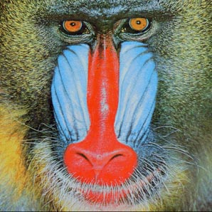
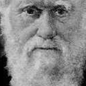
Data Compression
 |
Data Compression The textbook Algorithms, 4th Edition by Robert Sedgewick and Kevin Wayne surveys the most important algorithms and data structures in use today. The broad perspective taken makes it an appropriate introduction to the field. |
| Source: algs4.cs.princeton.edu/55compression/ | |
Data compression: reduces the size of a file to save space when storing it and to save time when transmitting it. Moore's law: # transistor on a chip doubles every 18-24 months. Parkinson's law: data expands to fill available space. Text, images, sound, video, etc. Wikipedia providespublic dumps of all content for academic research and republishing. Uses bzip and SevenZip's LZMA. Can take a week to compress of 300GB of data.
Ancient ideas.
Morse code, decimal number system, natural language, rotary phones (lower numbers were quicker to dial, so New York was 212 and Chicago 312).
Binary input and output streams.
We use BinaryStdIn.java, BinaryStdOut.java, BinaryDump.java, HexDump.java, and PictureDump.java.
Fixed length codes.
Need ceil(lg R) bits to specify one of R symbols. Genome.java. Uses Alphabet.java.
Run length encoding.
Variable-length codes.
Desire unique decodable codes. One way to achieve this is to append a special stop symbol to each codeword. Better approach: prefix-free codes: no string is a prefix of another. For example, { 01, 10, 0010, 1111 } is prefix free, but { 01, 10, 0010, 1010 } is not because 10 is a prefix of 1010.
Give fax machine example.
Huffman codes.
Specific way to construct optimal prefix-free codes. Invented by David Huffman while a student at MIT in 1950. Huffman.javaimplements Huffman algorithm.
Property A. No prefix free code uses fewer bits.
LZW compression.
Using prefix match code from TST.java, LZW.java implements LZW compression.
Real world: Pkzip = LZW + Shannon-Fano, GIF, TIFF, V.42bis modem, Unix compress. Practical issues:
- Encode everything in binary.
- Limit the number of elements in the symbol table (GIF = throw away and start over, Unix compress = throw away when not effective).
- Initially dictionary has 512 elements (with 256 elements filled in for ASCII characters), so we transmit 9 bits per integer. When it fills up, we double it to 1024 and start transmitting 10 bits per integer.
- Only traverse the tree once (might break our string table abstraction).
Practical issues: limit the number of elements in the symbol table.
Summary.
Huffman: variable length code for fixed length symbols. LZW: fixed length code for variable length strings.
Universal compression algorithm.
Impossible to compress all files (proof by simple counting argument). Intuitive argument: compress life work of Shakespeare, then compress result, then compress result again. If each file strictly shrinks, eventually you will be left with one bit.
References.
Guy Blelloch of CMU has an excellent chapter on data compression.
Error correction / detection.
Suppose channel for sending information is noisy and each bit gets flipped with probability p. Send each bit 3 times; to decode take the majority of the 3 bits. Decoded bit is correct with probability 3p^2 - 2p^3. This is less than p (if p < 1/2). Can reduce probability of decoding the bit incorrectly by sending each bit k times, but this is wasteful in terms of the transmission rate.
Reed-Solomon codes.
Reference. Used in mass storage systems (CDs and DVDs) and satellite transmissions (Voyager space probe, Mars Pathfinder) when the errors are bursty. Think of data to send as a degree d polynomial. Only need d+1 points to uniquely specify the polynomial. Send more points to enable error correction / detection. If code we want to send is a0, a1, ..., am-1 (each elements over finite field K), think of it as the polynomial p(x) = a0 + a1x + ... + am-1 x^m-1. Send p(0), p(b), p(b^2), ..., where b is a generator of multiplicative cyclic group over K.
Shannon's coding theorem.
Roughly speaking, if channel capacity is C, then we can send bits at a rate slightly less than C with an encoding scheme that will reduce probability of a decoding error to any desired level. Proof is nonconstructive.
Q+A
Exercises
- Which of the following codes are prefix free? Uniquely decodable? For those that are uniquely decodable, give the encoding of 1000000000000.
    code 1    code 2    code 3   code 4
A     0         0          1       1
B     100       1         01      01
C     10       00        001     001
D     11       11       0001     000
- Given an example of a uniquely-decodable code that is not prefix free.Solution. Any suffix-free code is uniquely decodable, e.g., { 0, 01 }.
- Given an example of a uniquely-decodable code that is not prefix free or suffix free.Solution. { 0011, 011, 11, 1110 } or { 01, 10, 011, 110 }.
- Are { 1, 100000, 00 }, { 01, 1001, 1011, 111, 1110 }, and { 1, 011, 01110, 1110, 10011 } uniquely decodable? If not, find a string with two encodings. Solution. The first set of codewords is uniquely decodable. The second set of codewords is not uniquely decodable because 111-01-1110-01 and 1110-111-1001 are two decodings of 11101111001. The third set of codewords ins not uniquely decodable because 01110-1110-011 and 011-1-011-10011 are two decodings of 011101110011.
- Test for uniquely decodability. Implement the Sardinas-Patterson algorithm for testing whether a set of codewords is uniquely decodable: Add all of the codewords to a set. Examine all pairs of codewords to see if any one is a prefix of another; if so, extract the dangling suffix (i.e., the part of the longer string that is not a prefix of the shorter one). If the dangling suffix is a codeword, then the code is not uniquely decodable; otherwise, add the dangling suffix to the list (provided it is not already there). Repeat this process with the larger list until there are no remaining new dangling suffix.The algorithm is finite because all dangling suffixes added to the list are suffixes of a finite set of codewords, and a dangling suffix can be added at most once.
- { 0, 01, 11 }. The codeword 0 is a prefix of 01, so add the dangling suffix 1. { 0, 01, 11, 1 }. The codeword 0 is a prefix of 01, but the dangling suffix 1 is already in the list; the codeword 1 is a prefix of 11, but the dangling suffix 1 is already in the list. There are no other dangling suffixes, so conclude that the set is uniquely decodable.
- { 0, 01, 10 }. The codeword 0 is a prefix of 01, so add the dangling suffix 1 to the list. { 0, 01, 10, 1 }. The codeword 1 is a prefix of 10, but the dangling suffix 0 is a codewords. So, conclude that the code is not uniquely decodeable.
- Kraft-McMillan inequality. Conside a code C with N codewords of lengths n1, n2, ..., nN. Prove that if the code is uniquely decodable, then K(C) = sum_i = 1 to N 2^(-ni) ≤ 1.
- Kraft-McMillan construction. Suppose that we have a set of integers n1, n2, ..., nN that satisfy the inequality sum_i = 1 to N 2^(-ni) ≤ 1. Prove that it is always possible to find a prefix-free code with codewords lengths n1, n2, ..., nN. Thus, by restricting attention to prefix-free codes (instead of uniquely decodable codes), we do not lose much.
- Kraft-McMillan equality for optimal prefix-free codes. Prove that if C is an optimal prefix-free code then the Kraft-McMillan inequality is an equality: K(C) = sum_i = 1 to N 2^(-ni) = 1.
- Suppose that all of the symbol probabilities are negative powers of 2. Describe the Huffman code.
- Suppose that all of the symbol frequencies are equal. Describe the Huffman code.
- Find a Huffman code where the length of a symbol with probability pi is greater than ceil(-lg pi).Solution. .01 (000), .30 (001), .34 (01), .35 (1). The codeword 001 has length greater than ceil(-lg .30).
- True or false. Any optimal prefix-free code can be obtained via Huffman's algorithm.Solution. False. Consider the following set of symbols and frequencies (A 26, B 24, C 14, D 13, E 12, F 11).
       C1   C2   C3
A 26   01   10   00
B 24   10   01   01
C 14  000  111  100
D 13  001  110  101
E 12  110  001  110
F 11  111  000  111
In any Huffman code, the codings for A and B must begin with different bits, but the code C3 does not have this property (yet it is an optimal prefix-free code).
- What is the LZW encoding of the following inputs?
- T O B E O R N O T T O B E
- Y A B B A D A B B A D A B B A D O O
- A A A A A A A A A A A A A A A A A A A A A
- Characterize the tricky situation in LZW coding.Solution. Whenever it encounteres cScSc, where c is a symbol, S is a string, cS is in the dictionary but cSc is not.
- As a function of N, how many bits are needed to encode N copies of the symbol A? N copies of the sequence ABC?
- Let F(i) be the ith Fibonacci number. Consider N symbols, where the ith symbol has frequency F(i). Note that F(1) + F(2) + ... + F(N) = F(N+2) - 1. Describe the Huffman code.Solution. Longest codeword has length N-1.
- Show that there are at least 2^(N-1) different Huffman codes corresponding to a given set of N symbols.Solution. There are N-1 internal nodes and each one has an arbitrary choice to assign its left and right children.
- Give a Huffman code where the frequency of 0s in the output is much much higher than the frequency of 1s.Solution. If the character 'A' occurs one million times and the character 'B' occurs once, the code word for 'A' will be 0 and the codeword for 'B' will be 1.
- Prove the following facts about Huffman tries.
- The two longest codewords have the same length.
- If the frequency of symbol i is strictly larger than the frequency of symbol j, then the length of the codeword for symbol i is less than or equal to the length of the codeword for symbol j.
- Describe how to transmit a Huffman code (or optimal prefix-free code) on a set of symbols { 0, 1, ..., N-1 } using 2N - 1 + N ceil(lg N) bits.Hint: use 2N-1 bits to specify the structure of the corresponding trie.
- Suppose that in an extended ASCII file (8-bit characters), the maximum character frequency is at most twice the minimum character frequency. Prove that and fixed-length 8-bit extended ASCII code is optimal.
- Shannon-Fano coding. Prove that the following top-down version of Huffman's algorithm is not optimal. Split the set of codewords C into two subsets C1 and C2 with (almost) equal frequencies. Recursively build the tree for C1 and C2, starting all codewords for C1 with 0 and all codewords for C2 with 1. To implement the first step, Shannon and Fano propose sorting the codewords by frequency and breaking the set up into two subarrays as best as possible.Solution. S 32, H 25, A 20, N 18, O 5.
- LZMW coding (Miller-Wegman 1985). LZ variant: search input for longest string already in the dictionary (the current match); add concatenation of previous match to current match to the dictionary. Dictionary entries grow more rapidly. Can also delete low-frequency entries when the dictionary fills up. Hard to implement.
- LZAP coding. Similar to LZMW: instead of adding just the concatenation of the previous match with the current match, add the concatenation of the previous match with all prefixes of the current match. Easier than LZMW to implement, but even more dictionary entries.
- Identify an optimal code that is not prefix-free.Hint: only need 3 symbols with equal frequencies.
- Identify two optimal prefix-free codes for the same input that have a different distribution of codeword lengths.Hint: only need 4 symbols.
- Minimum variance Huffman coding. Due to the nondeterminism associated with tiebraking, Huffman's algorithm may produce codes with different distributions of codeword lengths. When transmitting the compressed stream as it is being generated, it is desirable to transmit bits at a (near) constant rate. Find Huffman code that minimize sum_i (p_i (l_i - l_average(T)) ^2).Solution. When combining tries, break ties by picking the earliest produced trie with the smallest probability.
- Two-queue algorithm for Huffman coding. Prove that the following algorithm computes a Huffman code (and runs in linear time if the input symbols are already sorted by frequency). Maintain two FIFO queues: the first queue contains the input symbols, in ascending order of frequency, the second queue contains the internal nodes with combined weights. As long as there is more than one node in the two queues, dequeue the two nodes with the smallest weight by examining the fronts of both queues. Create a new internal node (left and right child = two nodes, weight = sum of weight of two nodes) and enqueue on the second queue.To obtain a minimum variance Huffman code, break ties by choosing nodes from the first queue.
Hint: prove that the second queue is sorted in ascending order of frequency.
- Sibling property. A binary tree has the sibling property if (i) every node (except the root) has a sibling and (ii) the binary tree can be listed in non-increasing order of probability such that, in the list, all siblings are adjacent. Prove that a binary tree represents a Huffman tree if and only if it has the sibling property.
- Relative coding. Instead of compressing each pixel in an image, consider the difference between a pixel and the previous one and encode the difference. Intuition: usually the pixels don't change much. Use with LZW over color table alphabet.
- Variable-width LZW codes. Increase the width of the table from p to p+1 after 2^p th codeword is inserted into table. Used with color table alphabet.
- Adaptive Huffman coding. One-pass algorithm and don't need to send prefix-free code. Build Huffman tree based on frequency of characters read in so far. Update tree after reading in each character. Encoder and decoder need to coordinate on tie-breaking conventions.
- Shannon entropy. The entropy H of a discrete random variable X with possible values x1, ..., xN that occur with probability p1, ..., pN is defined as H(X) = -p1 lg p1 - p2 lg p2 - ... - pN lg pN, where 0 lg 0 = 0 is consistent with the limit.
- What is the entropy of a fair coin?
- What is the entropy of a coin where both sides are heads?
- What is the entropy of a six-sided die?Solution. -lg (1/6) which is about 2.584962.
- What is the entropy of the sum of two fair dice?
- Given a random variable that takes on N values. What distribution maximizes the entropy?
The entropy is a fundamental concept in information theory. Shannon's source coding theorem asserts that to compress the data from a stream of independent and identically distributed random variables requires at least H(X) bits per symbol in the limit. For example, to send the results of a sequence of fair die tosses requires at least 2.584962 bits per die toss.
- Empirical entropy. The empirical entropy of a piece of text is obtained by computing the frequency of occurrence of each symbol and using these as the probabilities for a discrete random variable. Compute the empirical entropy of your favorite novel. Compare it to the data compression rate achieved by a Huffman code.
- Shannon experiment. Perform the following experiment. Give a subject a sequence of k letters from a piece of text (or Leipzig corpus) and ask them to predict the next letter. Estimate the fraction of times the subject gets the answer right for k = 1, 2, 5, 100.
- True or false. Fixed-length codes are uniquely decodable.Solution. True, they are prefix free.
- Give two different Huffman trees the string ABCCDD, with different heights.
- Prefix-free codes. Design an efficient algorithm to determine if a set of binary code words is prefix-free. Hint: use a binary trie or sort.
- Uniquely decodable code. Devise a uniquely decodable code that is not a prefix free code. Hint: suffix free codes = reverse of prefix free codes. Reverse of suffix free code is prefix free code -> can decode by reading compressed message in reverse order. Not very convenient.
- Huffman tree. Modify Huffman.java so that the encoder prints out the lookup table instead of the preorder traversal, and modify the decoder so that it constructs the tree by reading in the lookup table.
- True or false. In an optimal prefix-free ternary code, the three symbols that occur least frequently have the same length.Solution. False.
- Ternary Huffman codes. Generalize the Huffman algorithm to codewords over the ternary alphabet (0, 1, and 2) instead of the binary alphabet. That is, given a bytestream, find a prefix-free ternary code that uses as few trits (0s, 1s, and 2s) as possible. Prove that it yields optimal prefix-free ternary code.Solution. Combine smallest 3 probabilities at each step (instead of smallest 2). This works when there are 3 + 2k symbols for some integer k. To reduce to this case, add 1 or 2 dummy symbols of probability 0. (Alternatively, combine fewer than 3 symbols in the first step if the number of symbols is not 3 + 2k.) Ex: { 0.1, 0.2, 0.2, 0.5 }.
- Nonbinary Huffman codes. Extend the Huffman algorithm to codewords over the m-ary alphabet (0, 1, 2, ..., m-1) instead of the binary alphabet.
- Consider the following 21 character message that consists of 3 a's, 7c's, 6 t's and 5 g's.
a a c c c c a c t t g g g t t t t c c g g
Are the following 43 bits a possible Huffman encoding of the message above?
0000001111000101010010010010101010111001001
Justify your answer as concisely and rigorously as possible.Solution. A Huffman encoding for a message produces an encoding that uses the fewest bits among any prefix free code. The 2-bit binary code a = 00, c = 01, g = 10, t = 11 is a prefix free code that uses 21 * 2 = 42 bits. Thus, a Huffman code would use fewer than 43 bits.
- A binary tree is full if every node that is not a leaf has two children. Prove that any binary tree corresponding to an optimal prefix-free code is full.Hint: if an internal node has only one child, replace that internal node with its unique child.
- Move-to-front coding (Bentley, Sleator, Tarjan, and Wei 1986). Write a program MoveToFront that implements move-to-front encoding and decoding. Maintain alphabet of symbols in a list, where frequently occurring symbols are towards the front. A symbol is encoded as the number of symbols that precede it in the list. After encoding a symbol, move it to the front of the list. reference
- Move-ahead-k coding. Same as move-to-front coding, but move symbol k positions toward the front.
- Wait-c-and-move. Same as move-to-front coding, but move symbol to the front only after it has been encountered c times since the last time it was moved to the front.
- Double Huffman compression. Find an input for which applying the compress() method in Huffman.java twice leads to a strictly smaller output than applying compress() only once.
- Merging k sorted arrays. You have k sorted lists, of lenths n1, n2, ..., nk. Supposet that the only operation you can perform to combine lists is a 2-way merge: given one sorted array of length n1 and another sorted array of length n2, replace them with a sorted array of length n = n1 + n2. Moreover, the 2-way merge operation takes exactly n units of time. What is the optimal way to merge the k sorted arrays?Solution. Sort the list lengths so that n1 < n2 < ... < nk. Repetedly take the two smallest lists and apply the 2-way merge operation. The proof of optimality is the same as the proof of optimality of Huffman codes: repeatedly applying 2-way merge operations induces a binary tree in which each leaf node corresponds to one of the original sorted lists and each internal node corresponds to a 2-way merge operation. The contribution of any original list to the overall cost is the length of the list multiplied by its tree depth (because that is the number of times its elements are involved in a 2-way merge).
Strongly Connected Components
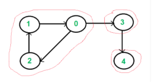
Birth control app

CACM Feb. 2015 - YFCC100M: The New Data in Multimedia Research HD
Inmutable Objects
![]()
Collected Java Practices
![]()
Skiena's Algo lectures
The real 10 algorithms

Shuffling algorithm analysis

Online Programming Visualizer
![]()
Nearly All Binary Searches and Mergesorts are Broken

027 - Example 01 - Coin Flip - Part 01 (Pseudocode)

13. Breadth-First Search (BFS)

Algo Visualizations
![]()
Data Structure Animations with Dr. Daniel Liang

Visualgo
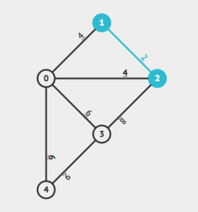
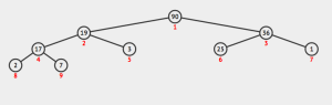
Intro to Algo from umd

Turing Machine

Cryptography Exercises
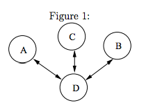
10 Codes and Ciphers

Curves and surfaces for computer graphics
Hash Functions
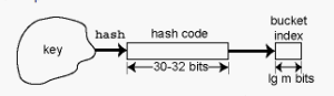
84 Skill & Expertise Endorsements (Ranked #13 out of 1.12M)

wiki books algorithms

Geeks for geeks

Michael Collins at Columbia

Machine Learning - Michael Collins

Design and analysis of algorithms
![]()
Animation tester
http://pages.cs.wisc.edu/~bahls/all/SortAnimation/sort/
Pancake sort Rosetta code
http://rosettacode.org/wiki/Sorting_algorithms/Pancake_sort#Java
Big O Notation

Binary Trees in Java - New Think Tank

Java Notes - Binary Trees