


The content for this post has been contributed by Quincy Smith, who is a part of the marketing team at Springboard an online training company seeking…


Unstructured data, especially text, images and videos contain a wealth of information. However, due to the inherent complexity in processing and analyzing this data, people often refrain from spending extra time and effort in venturing out from structured datasets to analyze these unstructured sources of data, which can be a potential gold mine.
Natural Language Processing (NLP) is all about leveraging tools, techniques and algorithms to process and understand natural language-based data, which is usually unstructured like text, speech and so on. In this series of articles, we will be looking at tried and tested strategies, techniques and workflows which can be leveraged by practitioners and data scientists to extract useful insights from text data. We will also cover some useful and interesting use-cases for NLP. This article will be all about processing and understanding text data with tutorials and hands-on examples.
The nature of this series will be a mix of theoretical concepts but with a focus on hands-on techniques and strategies covering a wide variety of NLP problems. Some of the major areas that we will be covering in this series of articles include the following.
Feel free to suggest more ideas as this series progresses, and I will be glad to cover something I might have missed out on. A lot of these articles will showcase tips and strategies which have worked well in real-world scenarios.
This article will be covering the following aspects of NLP in detail with hands-on examples.
This should give you a good idea of how to get started with analyzing syntax and semantics in text corpora.
Formally, NLP is a specialized field of computer science and artificial intelligence with roots in computational linguistics. It is primarily concerned with designing and building applications and systems that enable interaction between machines and natural languages that have been evolved for use by humans. Hence, often it is perceived as a niche area to work on. And people usually tend to focus more on machine learning or statistical learning.

When I started delving into the world of data science, even I was overwhelmed by the challenges in analyzing and modeling on text data. However, after working as a Data Scientist on several challenging problems around NLP over the years, I’ve noticed certain interesting aspects, including techniques, strategies and workflows which can be leveraged to solve a wide variety of problems. I have covered several topics around NLP in my books “Text Analytics with Python” (I’m writing a revised version of this soon) and “Practical Machine Learning with Python”.
However, based on all the excellent feedback I’ve received from all my readers (yes all you amazing people out there!), the main objective and motivation in creating this series of articles is to share my learnings with more people, who can’t always find time to sit and read through a book and can even refer to these articles on the go! Thus, there is no pre-requisite to buy any of these books to learn NLP.
When building the content and examples for this article, I was thinking if I should focus on a toy dataset to explain things better, or focus on an existing dataset from one of the main sources for data science datasets. Then I thought, why not build an end-to-end tutorial, where we scrape the web to get some text data and showcase examples based on that!
The source data which we will be working on will be news articles, which we have retrieved from inshorts, a website that gives us short, 60-word news articles on a wide variety of topics, and they even have an app for it!
In this article, we will be working with text data from news articles on technology, sports and world news. I will be covering some basics on how to scrape and retrieve these news articles from their website in the next section.
I am assuming you are aware of the CRISP-DM model, which is typically an industry standard for executing any data science project. Typically, any NLP-based problem can be solved by a methodical workflow that has a sequence of steps. The major steps are depicted in the following figure.
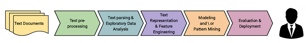
We usually start with a corpus of text documents and follow standard processes of text wrangling and pre-processing, parsing and basic exploratory data analysis. Based on the initial insights, we usually represent the text using relevant feature engineering techniques. Depending on the problem at hand, we either focus on building predictive supervised models or unsupervised models, which usually focus more on pattern mining and grouping. Finally, we evaluate the model and the overall success criteria with relevant stakeholders or customers, and deploy the final model for future usage.
We will be scraping inshorts, the website, by leveraging python to retrieve news articles. We will be focusing on articles on technology, sports and world affairs. We will retrieve one page’s worth of articles for each category. A typical news category landing page is depicted in the following figure, which also highlights the HTML section for the textual content of each article.

Thus, we can see the specific HTML tags which contain the textual content of each news article in the landing page mentioned above. We will be using this information to extract news articles by leveraging the BeautifulSoup and requests libraries. Let’s first load up the following dependencies.
import requests
from bs4 import BeautifulSoup
import pandas as pd
import numpy as np
import matplotlib.pyplot as plt
import seaborn as sns
import os
%matplotlib inline
We will now build a function which will leverage requests to access and get the HTML content from the landing pages of each of the three news categories. Then, we will use BeautifulSoup to parse and extract the news headline and article textual content for all the news articles in each category. We find the content by accessing the specific HTML tags and classes, where they are present (a sample of which I depicted in the previous figure).
It is pretty clear that we extract the news headline, article text and category and build out a data frame, where each row corresponds to a specific news article. We will now invoke this function and build our dataset.
news_df = build_dataset(seed_urls)
news_df.head(10)

We, now, have a neatly formatted dataset of news articles and you can quickly check the total number of news articles with the following code.
news_df.news_category.value_counts()Output:
-------
world         25
sports        25
technology    24
Name: news_category, dtype: int64
There are usually multiple steps involved in cleaning and pre-processing textual data. I have covered text pre-processing in detail in Chapter 3 of ‘Text Analytics with Python’ (code is open-sourced). However, in this section, I will highlight some of the most important steps which are used heavily in Natural Language Processing (NLP) pipelines and I frequently use them in my NLP projects. We will be leveraging a fair bit of nltk and spacy, both state-of-the-art libraries in NLP. Typically a pip install <library> or a conda install <library> should suffice. However, in case you face issues with loading up spacy’s language models, feel free to follow the steps highlighted below to resolve this issue (I had faced this issue in one of my systems).
# OPTIONAL: ONLY USE IF SPACY FAILS TO LOAD LANGUAGE MODEL
# Use the following command to install spaCy
> pip install -U spacyOR> conda install -c conda-forge spacy# Download the following language model and store it in disk
https://github.com/explosion/spacy-models/releases/tag/en_core_web_md-2.0.0# Link the same to spacy
> python -m spacy link ./spacymodels/en_core_web_md-2.0.0/en_core_web_md en_coreLinking successful
    ./spacymodels/en_core_web_md-2.0.0/en_core_web_md --> ./Anaconda3/lib/site-packages/spacy/data/en_coreYou can now load the model via spacy.load('en_core')
Let’s now load up the necessary dependencies for text pre-processing. We will remove negation words from stop words, since we would want to keep them as they might be useful, especially during sentiment analysis.
❗ IMPORTANT NOTE: A lot of you have messaged me about not being able to load the contractions module. It’s not a standard python module. We leverage a standard set of contractions available in the
contractions.pyfile in my repository.Please add it in the same directory you run your code from, else it will not work.
import spacy
import pandas as pd
import numpy as np
import nltk
from nltk.tokenize.toktok import ToktokTokenizer
import re
from bs4 import BeautifulSoup
from contractions import CONTRACTION_MAP
import unicodedatanlp = spacy.load('en_core', parse=True, tag=True, entity=True)
#nlp_vec = spacy.load('en_vecs', parse = True, tag=True, #entity=True)
tokenizer = ToktokTokenizer()
stopword_list = nltk.corpus.stopwords.words('english')
stopword_list.remove('no')
stopword_list.remove('not')
Often, unstructured text contains a lot of noise, especially if you use techniques like web or screen scraping. HTML tags are typically one of these components which don’t add much value towards understanding and analyzing text.
'Some important text'
It is quite evident from the above output that we can remove unnecessary HTML tags and retain the useful textual information from any document.
Usually in any text corpus, you might be dealing with accented characters/letters, especially if you only want to analyze the English language. Hence, we need to make sure that these characters are converted and standardized into ASCII characters. A simple example — converting éto e.
'Some Accented text'
The preceding function shows us how we can easily convert accented characters to normal English characters, which helps standardize the words in our corpus.
Contractions are shortened version of words or syllables. They often exist in either written or spoken forms in the English language. These shortened versions or contractions of words are created by removing specific letters and sounds. In case of English contractions, they are often created by removing one of the vowels from the word. Examples would be, do not to don’t and I would to I’d. Converting each contraction to its expanded, original form helps with text standardization.
We leverage a standard set of contractions available in the
contractions.pyfile in my repository.
'You all cannot expand contractions I would think'
We can see how our function helps expand the contractions from the preceding output. Are there better ways of doing this? Definitely! If we have enough examples, we can even train a deep learning model for better performance.
Special characters and symbols are usually non-alphanumeric characters or even occasionally numeric characters (depending on the problem), which add to the extra noise in unstructured text. Usually, simple regular expressions (regexes) can be used to remove them.
'Well this was fun What do you think '
I’ve kept removing digits as optional, because often we might need to keep them in the pre-processed text.
To understand stemming, you need to gain some perspective on what word stems represent. Word stems are also known as the base form of a word, and we can create new words by attaching affixes to them in a process known as inflection. Consider the word JUMP. You can add affixes to it and form new words like JUMPS, JUMPED, and JUMPING. In this case, the base word JUMP is the word stem.

The figure shows how the word stem is present in all its inflections, since it forms the base on which each inflection is built upon using affixes. The reverse process of obtaining the base form of a word from its inflected form is known as stemming. Stemming helps us in standardizing words to their base or root stem, irrespective of their inflections, which helps many applications like classifying or clustering text, and even in information retrieval. Let’s see the popular Porter stemmer in action now!
'My system keep crash hi crash yesterday, our crash daili'
The Porter stemmer is based on the algorithm developed by its inventor, Dr. Martin Porter. Originally, the algorithm is said to have had a total of five different phases for reduction of inflections to their stems, where each phase has its own set of rules.
Do note that usually stemming has a fixed set of rules, hence, the root stems may not be lexicographically correct. Which means, the stemmed words may not be semantically correct, and might have a chance of not being present in the dictionary (as evident from the preceding output).
Lemmatization is very similar to stemming, where we remove word affixes to get to the base form of a word. However, the base form in this case is known as the root word, but not the root stem. The difference being that the root word is always a lexicographically correct word (present in the dictionary), but the root stem may not be so. Thus, root word, also known as the lemma, will always be present in the dictionary. Both nltk and spacyhave excellent lemmatizers. We will be using spacy here.
'My system keep crash ! his crash yesterday , ours crash daily'
You can see that the semantics of the words are not affected by this, yet our text is still standardized.
Do note that the lemmatization process is considerably slower than stemming, because an additional step is involved where the root form or lemma is formed by removing the affix from the word if and only if the lemma is present in the dictionary.
Words which have little or no significance, especially when constructing meaningful features from text, are known as stopwords or stop words. These are usually words that end up having the maximum frequency if you do a simple term or word frequency in a corpus. Typically, these can be articles, conjunctions, prepositions and so on. Some examples of stopwords are a, an, the, and the like.
', , stopwords , computer not'
There is no universal stopword list, but we use a standard English language stopwords list from nltk. You can also add your own domain-specific stopwords as needed.
While we can definitely keep going with more techniques like correcting spelling, grammar and so on, let’s now bring everything we learnt together and chain these operations to build a text normalizer to pre-process text data.
Let’s now put this function in action! We will first combine the news headline and the news article text together to form a document for each piece of news. Then, we will pre-process them.
{'clean_text': 'us unveils world powerful supercomputer beat china us unveil world powerful supercomputer call summit beat previous record holder china sunway taihulight peak performance trillion calculation per second twice fast sunway taihulight capable trillion calculation per second summit server reportedly take size two tennis court', 'full_text': "US unveils world's most powerful supercomputer, beats China. The US has unveiled the world's most powerful supercomputer called 'Summit', beating the previous record-holder China's Sunway TaihuLight. With a peak performance of 200,000 trillion calculations per second, it is over twice as fast as Sunway TaihuLight, which is capable of 93,000 trillion calculations per second. Summit has 4,608 servers, which reportedly take up the size of two tennis courts."}
Thus, you can see how our text pre-processor helps in pre-processing our news articles! After this, you can save this dataset to disk if needed, so that you can always load it up later for future analysis.
news_df.to_csv('news.csv', index=False, encoding='utf-8')
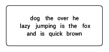
For any language, syntax and structure usually go hand in hand, where a set of specific rules, conventions, and principles govern the way words are combined into phrases; phrases get combines into clauses; and clauses get combined into sentences. We will be talking specifically about the English language syntax and structure in this section. In English, words usually combine together to form other constituent units. These constituents include words, phrases, clauses, and sentences. Considering a sentence,“The brown fox is quick and he is jumping over the lazy dog”, it is made of a bunch of words and just looking at the words by themselves don’t tell us much.
Knowledge about the structure and syntax of language is helpful in many areas like text processing, annotation, and parsing for further operations such as text classification or summarization. Typical parsing techniques for understanding text syntax are mentioned below.
We will be looking at all of these techniques in subsequent sections. Considering our previous example sentence “The brown fox is quick and he is jumping over the lazy dog”, if we were to annotate it using basic POS tags, it would look like the following figure.

Thus, a sentence typically follows a hierarchical structure consisting the following components,
sentence → clauses → phrases → words
Parts of speech (POS) are specific lexical categories to which words are assigned, based on their syntactic context and role. Usually, words can fall into one of the following major categories.
Besides these four major categories of parts of speech , there are other categories that occur frequently in the English language. These include pronouns, prepositions, interjections, conjunctions, determiners, and many others. Furthermore, each POS tag like the noun (N) can be further subdivided into categories like singular nouns (NN), singular proper nouns(NNP), and plural nouns (NNS).
The process of classifying and labeling POS tags for words called parts of speech tagging or POS tagging . POS tags are used to annotate words and depict their POS, which is really helpful to perform specific analysis, such as narrowing down upon nouns and seeing which ones are the most prominent, word sense disambiguation, and grammar analysis. We will be leveraging both nltk and spacy which usually use the Penn Treebank notation for POS tagging.

We can see that each of these libraries treat tokens in their own way and assign specific tags for them. Based on what we see, spacy seems to be doing slightly better than nltk.
Based on the hierarchy we depicted earlier, groups of words make up phrases. There are five major categories of phrases:
Shallow parsing, also known as light parsing or chunking , is a popular natural language processing technique of analyzing the structure of a sentence to break it down into its smallest constituents (which are tokens such as words) and group them together into higher-level phrases. This includes POS tags as well as phrases from a sentence.

We will leverage the conll2000 corpus for training our shallow parser model. This corpus is available in nltk with chunk annotations and we will be using around 10K records for training our model. A sample annotated sentence is depicted as follows.
10900 48
(S
  Chancellor/NNP
  (PP of/IN)
  (NP the/DT Exchequer/NNP)
  (NP Nigel/NNP Lawson/NNP)
  (NP 's/POS restated/VBN commitment/NN)
  (PP to/TO)
  (NP a/DT firm/NN monetary/JJ policy/NN)
  (VP has/VBZ helped/VBN to/TO prevent/VB)
  (NP a/DT freefall/NN)
  (PP in/IN)
  (NP sterling/NN)
  (PP over/IN)
  (NP the/DT past/JJ week/NN)
  ./.)
From the preceding output, you can see that our data points are sentences that are already annotated with phrases and POS tags metadata that will be useful in training our shallow parser model. We will leverage two chunking utility functions, tree2conlltags , to get triples of word, tag, and chunk tags for each token, and conlltags2tree to generate a parse tree from these token triples. We will be using these functions to train our parser. A sample is depicted below.
[('Chancellor', 'NNP', 'O'),
 ('of', 'IN', 'B-PP'),
 ('the', 'DT', 'B-NP'),
 ('Exchequer', 'NNP', 'I-NP'),
 ('Nigel', 'NNP', 'B-NP'),
 ('Lawson', 'NNP', 'I-NP'),
 ("'s", 'POS', 'B-NP'),
 ('restated', 'VBN', 'I-NP'),
 ('commitment', 'NN', 'I-NP'),
 ('to', 'TO', 'B-PP'),
 ('a', 'DT', 'B-NP'),
 ('firm', 'NN', 'I-NP'),
 ('monetary', 'JJ', 'I-NP'),
 ('policy', 'NN', 'I-NP'),
 ('has', 'VBZ', 'B-VP'),
 ('helped', 'VBN', 'I-VP'),
 ('to', 'TO', 'I-VP'),
 ('prevent', 'VB', 'I-VP'),
 ('a', 'DT', 'B-NP'),
 ('freefall', 'NN', 'I-NP'),
 ('in', 'IN', 'B-PP'),
 ('sterling', 'NN', 'B-NP'),
 ('over', 'IN', 'B-PP'),
 ('the', 'DT', 'B-NP'),
 ('past', 'JJ', 'I-NP'),
 ('week', 'NN', 'I-NP'),
 ('.', '.', 'O')]
The chunk tags use the IOB format. This notation represents Inside, Outside, and Beginning. The B- prefix before a tag indicates it is the beginning of a chunk, and I- prefix indicates that it is inside a chunk. The O tag indicates that the token does not belong to any chunk. The B- tag is always used when there are subsequent tags of the same type following it without the presence of O tags between them.
We will now define a function conll_tag_ chunks() to extract POS and chunk tags from sentences with chunked annotations and a function called combined_taggers() to train multiple taggers with backoff taggers (e.g. unigram and bigram taggers)
We will now define a class NGramTagChunker that will take in tagged sentences as training input, get their (word, POS tag, Chunk tag) WTC triples, and train a BigramTagger with a UnigramTagger as the backoff tagger. We will also define a parse() function to perform shallow parsing on new sentences
The
UnigramTagger,BigramTagger, andTrigramTaggerare classes that inherit from the base classNGramTagger, which itself inherits from theContextTaggerclass , which inherits from theSequentialBackoffTaggerclass .
We will use this class to train on the conll2000 chunked train_data and evaluate the model performance on the test_data
ChunkParse score:
    IOB Accuracy:  90.0%%
    Precision:     82.1%%
    Recall:        86.3%%
    F-Measure:     84.1%%
Our chunking model gets an accuracy of around 90% which is quite good! Let’s now leverage this model to shallow parse and chunk our sample news article headline which we used earlier, “US unveils world’s most powerful supercomputer, beats China”.
chunk_tree = ntc.parse(nltk_pos_tagged)
print(chunk_tree)Output:
-------
(S
  (NP US/NNP)
  (VP unveils/VBZ world's/VBZ)
  (NP most/RBS powerful/JJ supercomputer,/JJ beats/NNS China/NNP))
Thus you can see it has identified two noun phrases (NP) and one verb phrase (VP) in the news article. Each word’s POS tags are also visible. We can also visualize this in the form of a tree as follows. You might need to install ghostscript in case nltk throws an error.
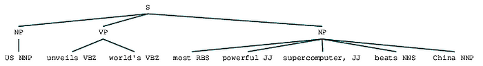
The preceding output gives a good sense of structure after shallow parsing the news headline.
Constituent-based grammars are used to analyze and determine the constituents of a sentence. These grammars can be used to model or represent the internal structure of sentences in terms of a hierarchically ordered structure of their constituents. Each and every word usually belongs to a specific lexical category in the case and forms the head word of different phrases. These phrases are formed based on rules called phrase structure rules.
Phrase structure rules form the core of constituency grammars, because they talk about syntax and rules that govern the hierarchy and ordering of the various constituents in the sentences. These rules cater to two things primarily.
The generic representation of a phrase structure rule is S → AB , which depicts that the structure S consists of constituents A and B , and the ordering is A followed by B . While there are several rules (refer to Chapter 1, Page 19: Text Analytics with Python, if you want to dive deeper), the most important rule describes how to divide a sentence or a clause. The phrase structure rule denotes a binary division for a sentence or a clause as S → NP VP where S is the sentence or clause, and it is divided into the subject, denoted by the noun phrase (NP) and the predicate, denoted by the verb phrase (VP).
A constituency parser can be built based on such grammars/rules, which are usually collectively available as context-free grammar (CFG) or phrase-structured grammar. The parser will process input sentences according to these rules, and help in building a parse tree.

We will be using nltk and the StanfordParser here to generate parse trees.
Prerequisites: Download the official Stanford Parser from here, which seems to work quite well. You can try out a later version by going to this website and checking the Release History section. After downloading, unzip it to a known location in your filesystem. Once done, you are now ready to use the parser from
nltk, which we will be exploring soon.
The Stanford parser generally uses a PCFG (probabilistic context-free grammar) parser. A PCFG is a context-free grammar that associates a probability with each of its production rules. The probability of a parse tree generated from a PCFG is simply the production of the individual probabilities of the productions used to generate it.
(ROOT
  (SINV
    (S
      (NP (NNP US))
      (VP
        (VBZ unveils)
        (NP
          (NP (NN world) (POS 's))
          (ADJP (RBS most) (JJ powerful))
          (NN supercomputer))))
    (, ,)
    (VP (VBZ beats))
    (NP (NNP China))))
We can see the constituency parse tree for our news headline. Let’s visualize it to understand the structure better.
from IPython.display import display
display(result[0])
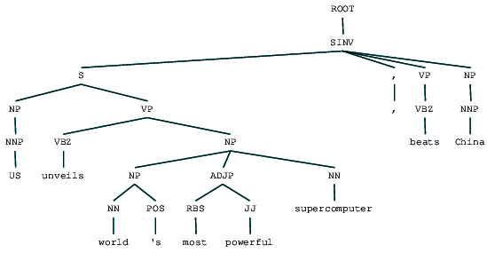
We can see the nested hierarchical structure of the constituents in the preceding output as compared to the flat structure in shallow parsing. In case you are wondering what SINV means, it represents an Inverted declarative sentence, i.e. one in which the subject follows the tensed verb or modal. Refer to the Penn Treebank reference as needed to lookup other tags.
In dependency parsing, we try to use dependency-based grammars to analyze and infer both structure and semantic dependencies and relationships between tokens in a sentence. The basic principle behind a dependency grammar is that in any sentence in the language, all words except one, have some relationship or dependency on other words in the sentence. The word that has no dependency is called the root of the sentence. The verb is taken as the root of the sentence in most cases. All the other words are directly or indirectly linked to the root verb using links , which are the dependencies.
Considering our sentence “The brown fox is quick and he is jumping over the lazy dog” , if we wanted to draw the dependency syntax tree for this, we would have the structure

These dependency relationships each have their own meaning and are a part of a list of universal dependency types. This is discussed in an original paper, Universal Stanford Dependencies: A Cross-Linguistic Typology by de Marneffe et al, 2014). You can check out the exhaustive list of dependency types and their meanings here.
If we observe some of these dependencies, it is not too hard to understand them.
fox → the and dog → the.fox → brown and dog → lazy.is → fox and jumping → he.is → and and is → jumping.jumping → is.is → quickjumping → over.over → dog.Spacy had two types of English dependency parsers based on what language models you use, you can find more details here. Based on language models, you can use the Universal Dependencies Scheme or the CLEAR Style Dependency Scheme also available in NLP4J now. We will now leverage spacy and print out the dependencies for each token in our news headline.
[]<---US[compound]--->[]
--------
['US']<---unveils[nsubj]--->['supercomputer', ',']
--------
[]<---world[poss]--->["'s"]
--------
[]<---'s[case]--->[]
--------
[]<---most[amod]--->[]
--------
[]<---powerful[compound]--->[]
--------
['world', 'most', 'powerful']<---supercomputer[appos]--->[]
--------
[]<---,[punct]--->[]
--------
['unveils']<---beats[ROOT]--->['China']
--------
[]<---China[dobj]--->[]
--------
It is evident that the verb beats is the ROOT since it doesn’t have any other dependencies as compared to the other tokens. For knowing more about each annotation you can always refer to the CLEAR dependency scheme. We can also visualize the above dependencies in a better way.

You can also leverage nltk and the StanfordDependencyParser to visualize and build out the dependency tree. We showcase the dependency tree both in its raw and annotated form as follows.
(beats (unveils US (supercomputer (world 's) (powerful most)))
 China)

You can notice the similarities with the tree we had obtained earlier. The annotations help with understanding the type of dependency among the different tokens.
In any text document, there are particular terms that represent specific entities that are more informative and have a unique context. These entities are known as named entities , which more specifically refer to terms that represent real-world objects like people, places, organizations, and so on, which are often denoted by proper names. A naive approach could be to find these by looking at the noun phrases in text documents. Named entity recognition (NER) , also known as entity chunking/extraction , is a popular technique used in information extraction to identify and segment the named entities and classify or categorize them under various predefined classes.
SpaCy has some excellent capabilities for named entity recognition. Let’s try and use it on one of our sample news articles.
[(US, 'GPE'), (China, 'GPE'), (US, 'GPE'), (China, 'GPE'),
 (Sunway, 'ORG'), (TaihuLight, 'ORG'), (200,000, 'CARDINAL'),
 (second, 'ORDINAL'), (Sunway, 'ORG'), (TaihuLight, 'ORG'),
 (93,000, 'CARDINAL'), (4,608, 'CARDINAL'), (two, 'CARDINAL')]

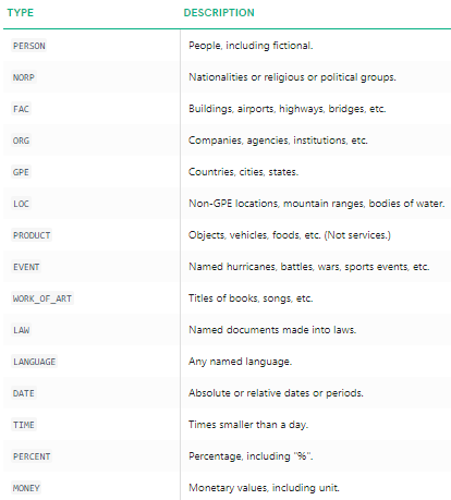
We can clearly see that the major named entities have been identified by spacy. To understand more in detail about what each named entity means, you can refer to the documentation or check out the following table for convenience.
Let’s now find out the most frequent named entities in our news corpus! For this, we will build out a data frame of all the named entities and their types using the following code.
We can now transform and aggregate this data frame to find the top occuring entities and types.

Do you notice anything interesting? (Hint: Maybe the supposed summit between Trump and Kim Jong!). We also see that it has correctly identified ‘Messenger’ as a product (from Facebook).
We can also group by the entity types to get a sense of what types of entites occur most in our news corpus.

We can see that people, places and organizations are the most mentioned entities though interestingly we also have many other entities.
Another nice NER tagger is the StanfordNERTagger available from the nltkinterface. For this, you need to have Java installed and then download the Stanford NER resources. Unzip them to a location of your choice (I used E:/stanford in my system).
Stanford’s Named Entity Recognizer is based on an implementation of linear chain Conditional Random Field (CRF) sequence models. Unfortunately this model is only trained on instances of PERSON, ORGANIZATION and LOCATION types. Following code can be used as a standard workflow which helps us extract the named entities using this tagger and show the top named entities and their types (extraction differs slightly from spacy).

We notice quite similar results though restricted to only three types of named entities. Interestingly, we see a number of mentioned of several people in various sports.
Sentiment analysis is perhaps one of the most popular applications of NLP, with a vast number of tutorials, courses, and applications that focus on analyzing sentiments of diverse datasets ranging from corporate surveys to movie reviews. The key aspect of sentiment analysis is to analyze a body of text for understanding the opinion expressed by it. Typically, we quantify this sentiment with a positive or negative value, called polarity. The overall sentiment is often inferred as positive, neutral or negative from the sign of the polarity score.
Usually, sentiment analysis works best on text that has a subjective context than on text with only an objective context. Objective text usually depicts some normal statements or facts without expressing any emotion, feelings, or mood. Subjective text contains text that is usually expressed by a human having typical moods, emotions, and feelings. Sentiment analysis is widely used, especially as a part of social media analysis for any domain, be it a business, a recent movie, or a product launch, to understand its reception by the people and what they think of it based on their opinions or, you guessed it, sentiment!

Typically, sentiment analysis for text data can be computed on several levels, including on an individual sentence level, paragraph level, or the entire document as a whole. Often, sentiment is computed on the document as a whole or some aggregations are done after computing the sentiment for individual sentences. There are two major approaches to sentiment analysis.
For the first approach we typically need pre-labeled data. Hence, we will be focusing on the second approach. For a comprehensive coverage of sentiment analysis, refer to Chapter 7: Analyzing Movie Reviews Sentiment, Practical Machine Learning with Python, Springer\Apress, 2018. In this scenario, we do not have the convenience of a well-labeled training dataset. Hence, we will need to use unsupervised techniques for predicting the sentiment by using knowledgebases, ontologies, databases, and lexicons that have detailed information, specially curated and prepared just for sentiment analysis. A lexicon is a dictionary, vocabulary, or a book of words. In our case, lexicons are special dictionaries or vocabularies that have been created for analyzing sentiments. Most of these lexicons have a list of positive and negative polar words with some score associated with them, and using various techniques like the position of words, surrounding words, context, parts of speech, phrases, and so on, scores are assigned to the text documents for which we want to compute the sentiment. After aggregating these scores, we get the final sentiment.

Various popular lexicons are used for sentiment analysis, including the following.
This is not an exhaustive list of lexicons that can be leveraged for sentiment analysis, and there are several other lexicons which can be easily obtained from the Internet. Feel free to check out each of these links and explore them. We will be covering two techniques in this section.
The AFINN lexicon is perhaps one of the simplest and most popular lexicons that can be used extensively for sentiment analysis. Developed and curated by Finn Årup Nielsen, you can find more details on this lexicon in the paper, “A new ANEW: evaluation of a word list for sentiment analysis in microblogs”, proceedings of the ESWC 2011 Workshop. The current version of the lexicon is AFINN-en-165. txt and it contains over 3,300+ words with a polarity score associated with each word. You can find this lexicon at the author’s official GitHub repository along with previous versions of it, includingAFINN-111. The author has also created a nice wrapper library on top of this in Python called afinn, which we will be using for our analysis.
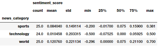
The following code computes sentiment for all our news articles and shows summary statistics of general sentiment per news category.

We can get a good idea of general sentiment statistics across different news categories. Looks like the average sentiment is very positive in sports and reasonably negative in technology! Let’s look at some visualizations now.
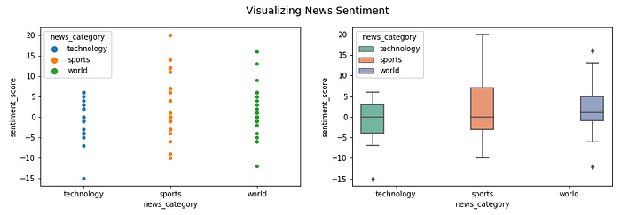
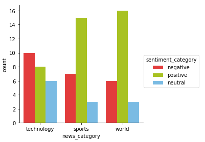
We can see that the spread of sentiment polarity is much higher in sportsand world as compared to technology where a lot of the articles seem to be having a negative polarity. We can also visualize the frequency of sentiment labels.
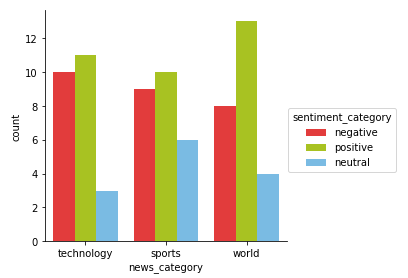
No surprises here that technology has the most number of negative articles and world the most number of positive articles. Sports might have more neutral articles due to the presence of articles which are more objective in nature (talking about sporting events without the presence of any emotion or feelings). Let’s dive deeper into the most positive and negative sentiment news articles for technology news.

Looks like the most negative article is all about a recent smartphone scam in India and the most positive article is about a contest to get married in a self-driving shuttle. Interesting! Let’s do a similar analysis for world news.
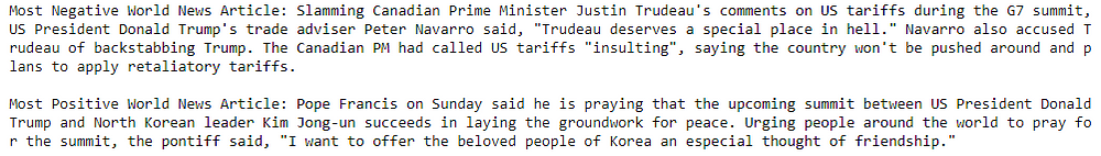
Interestingly Trump features in both the most positive and the most negative world news articles. Do read the articles to get some more perspective into why the model selected one of them as the most negative and the other one as the most positive (no surprises here!).
TextBlob is another excellent open-source library for performing NLP tasks with ease, including sentiment analysis. It also an a sentiment lexicon (in the form of an XML file) which it leverages to give both polarity and subjectivity scores. Typically, the scores have a normalized scale as compare to Afinn. The polarity score is a float within the range [-1.0, 1.0]. The subjectivity is a float within the range [0.0, 1.0] where 0.0 is very objective and 1.0 is very subjective. Let’s use this now to get the sentiment polarity and labels for each news article and aggregate the summary statistics per news category.
Looks like the average sentiment is the most positive in world and least positive in technology! However, these metrics might be indicating that the model is predicting more articles as positive. Let’s look at the sentiment frequency distribution per news category.
There definitely seems to be more positive articles across the news categories here as compared to our previous model. However, still looks like technology has the most negative articles and world, the most positive articles similar to our previous analysis. Let’s now do a comparative analysis and see if we still get similar articles in the most positive and negative categories for world news.

Well, looks like the most negative world news article here is even more depressing than what we saw the last time! The most positive article is still the same as what we had obtained in our last model.
Finally, we can even evaluate and compare between these two models as to how many predictions are matching and how many are not (by leveraging a confusion matrix which is often used in classification). We leverage our nifty model_evaluation_utils module for this.

In the preceding table, the ‘Actual’ labels are predictions from the Afinnsentiment analyzer and the ‘Predicted’ labels are predictions from TextBlob. Looks like our previous assumption was correct. TextBlob definitely predicts several neutral and negative articles as positive. Overall most of the sentiment predictions seem to match, which is good!
This was definitely one of my longer articles! If you are reading this, I really commend your efforts for staying with me till the end of this article. These examples should give you a good idea about how to start working with a corpus of text documents and popular strategies for text retrieval, pre-processing, parsing, understanding structure, entities and sentiment. We will be covering feature engineering and representation techniques with hands-on examples in the next article of this series. Stay tuned!
All the code and datasets used in this article can be accessed from my GitHub
The code is also available as a Jupyter notebook
I often mentor and help students at Springboard to learn essential skills around Data Science. Thanks to them for helping me develop this content. Do check out Springboard’s DSC bootcamp if you are interested in a career-focused structured path towards learning Data Science.
A lot of this code comes from the research and work that I had done during writing my book “Text Analytics with Python”. The code is open-sourced on GitHub. (Python 3.x edition coming by end of this year!)
“Practical Machine Learning with Python”, my other book also covers text classification and sentiment analysis in detail. The code is open-sourced on GitHub for your convenience.
If you have any feedback, comments or interesting insights to share about my article or data science in general, feel free to reach out to me on my LinkedIn social media channel.
Thanks to Durba for editing this article.

WRITTEN BY
This post assumes you have some basic knowledge of probability and statistics. If you don’t, do not be afraid, I have gathered a list of the best resources I could find to introduce you to these subjects, so that you can read this post, understand it, and enjoy it to its fullest.
In it, we will talk about one of the most famous and utilised theorems of probability theory: Bayes’ Theorem. Never heard about it? Then you are in for a treat! Know what it is already? Then read on to consolidate your knowledge with an easy, everyday example, so that you too can explain it in simple terms to others.
In the following posts we will learn about some simplifications of Baye’s theorem that are more practical, and about other probabilistic approaches to machine learning like Hidden Markov Models.
Lets go!
In this section I have listed three very good and concise (the two first mainly, the third one is a bit more extensive) sources to learn the basics of probability that you will need to understand this post. Don’t be afraid, the concepts are very simple and with a quick read you will most definitely understand them.
If you already have a grasp of basic probability, feel free to skip this section.
Okay, now you are ready to continue on with the rest of the post, sit back, relax, and enjoy.
Thomas Bayes (1701 — 1761) was an English theologian and mathematician that belonged to the Royal Society (the oldest national scientific society in the world and the leading national organisation for the promotion of scientific research in Britain), where other eminent individuals have enrolled, like Newton, Darwin or Faraday. He developed one of the most important theorems of probability, which coined his name: Bayes’ Theorem, or the Theorem of Conditional Probability.

To explain this theorem, we will use a very simple example. Imagine you have been diagnosed with a very rare disease, which only affects 0.1% of the population; that is, 1 in every 1000 persons.
The test you have taken to check for the disease correctly classifies 99% of the people who have the disease, incorrectly classifying healthy individuals with a 1% chance.
I am doomed! Is this disease fatal doctor?
Is what most people would say. However, after this test, what are the chances we have of actually suffering the disease?
99% for sure! I better get my stuff in order.
Upon this thought, Bayes’ mentality ought to prevail, as it is actually very far off from reality. Lets use Bayes’ Theorem to gain some perspective.
Bayes’ Theorem, or as I have called it before, the Theorem of Conditional Probability, is used for calculating the probability of a hypothesis (H) being true (ie. having the disease) given that a certain event (E) has happened (being diagnosed positive of this disease in the test). This calculation is described using the following formulation:


The term on the left of the equal sign P(H |E )is the probability of having the disease (H) given that we have been diagnosed positive (E) in a test for such disease, which is what we actually want to calculate. The vertical bars (|) in a probability term denote a conditional probability (ie, the probability of A given B would be P(A|B)).
The left term of the numerator on the right side P(E|H) is the probability of the event, given that the hypothesis is true. In our example this would be the probability of being diagnosed positive in the test, given that we have the disease.
The term next to it; P(H) is the prior probability of the hypothesis before any event has taken place. In this case it would be the probability of having the disease before any test has been taken.
Lastly, the term on the denominator; P(E) is the probability of the event, that is, the probability of being diagnosed positive for the disease. This term can be further decomposed into the sum of two smaller terms: having the disease and testing positive plus not having the disease and testing positive too.


In this formula P(~H) denotes the prior probability of not having the disease, where ~ means negation or not. The following picture describes each of the terms involved in the overall calculation of the conditional probability:


Remember, for us the hypothesis or assumption H is having the disease, and the event or evidence E is being diagnosed positive in the test for such disease.
If we use the first formula we saw (the complete formula for calculating the conditional probability of having the disease and being diagnosed positive), decompose the denominator, and insert in the numbers, we get the following calculation:


The 0,99 comes from the 99% probability of being diagnosed positive given that we have the disease, the 0,001 comes from the 1 in 1000 chance of having the disease, the 0,999 comes from the probability of not having this disease, and the last 0,01 comes from the probability of being diagnosed positive by the test even tough we do not have the disease. The final result of this calculation is:


9%! There is only a 9% chance that we have the disease! “How can this be?” you are probably asking yourself. Magic? No, my friends, it is not magic, it is just probability: common sense applied to mathematics. Like described in the book Thinking, Fast and Slow by Daniel Kahneman, the human mind is very bad at estimating and calculating probabilities, like it has been shown with the previous example, so we should always hold back our intuition, take a step back and use all the probability tools at our disposal.
Imagine now, that after being diagnosed positive on the first test, we decide to take another test with the same conditions, in a different clinic to double-check the results, and unluckily we get a positive diagnosis again, indicating that the second test also says that we have the disease.
What is the actual probability of having the disease now? Well, we can use exactly the same formula as before, but replacing the initial prior probability (0.1% chance of having the disease) with the posterior probability obtained the previous time (9% chance after being diagnosed positive by the test once), and their complementary terms.
If we crunch the numbers we get:


Now we have a much higher chance, 91% of actually having the disease. As bad as it might look tough, after two positive tests it is still not completely certain that we have the disease. Certainty seems to escape the world of probability.
The intuition behind this famous theorem is that we can never be fully certain of the world, as it is a changing being, change is in the nature of reality. However, something that we can do, which is the fundamental principle behind this theorem, is update and improve our knowledge of reality as we get more and more data or evidence.
This can be illustrated with a very simple example. Imagine the following situation: you are in the edge square shaped garden, sitting on a chair, looking outside the garden. On the opposite side, lies a servant that throws a initial blue ball inside the square. After that, he keeps throwing other yellow balls inside the square, and telling you where they land relatively to the initial green ball.

As more and more yellow balls land, and you get informed of where they land relative to the first blue ball, you gradually increase your knowledge of where the blue ball might be, leaving out certain parts of the garden: as we get more evidence (more yellow balls) we update our knowledge (the position of the blue ball).
In the example above, with only 3 yellow balls thrown, we could already start to build a certain idea that the blue ball lies somewhere within the top left corner of the garden.
When Bayes’ first formulated this theorem, he didn’t publish it at first, thinking it was nothing extraordinary, and the papers where the theorem was formulated were found after his death.
Today Bayes’ theorem is not only one of the bases of modern probability, but a highly used tool in many intelligent systems like spam filters, and many other text and non text related problem solvers.
In the following post we will see what these applications are, and how Bayes’ theorem and its variations can be applied to many real world use cases. To check it out follow me on Medium, and stay tuned!

That is all, I hope you liked the post. Feel Free to connect with me on LinkedIn or follow me on Twitter at @jaimezorno. Also, you can take a look at my other posts on Data Science and Machine Learning here. Have a good read!