Monte Carlo Simulation

https://introcs.cs.princeton.edu/java/98simulation/

This section under major construction.

In 1953 Enrico Fermi, John Pasta, and Stanslaw Ulam created the first "computer experiment" to study a vibrarting atomic lattice. Nonlinear system couldn't be analyzed by classical mathematics.

Simulation = analytic method that imitates a physical system. Monte Carlo simulation = use randomly generated values for uncertain variables. Named after famous casino in Monaco. At essentially each step in the evolution of the calculation, Repeat several times to generate range of possible scenarios, and average results. Widely applicable brute force solution. Computationally intensive, so use when other techniques fail. Typically, accuracy is proportional to square root of number of repetitions. Such techniques are widely applied in various domains including: designing nuclear reactors, predicting the evolution of stars, forecasting the stock market, etc.

Generating random numbers. The math library function Math.random generate a pseudo-random number greater than or equal to 0.0 and less than 1.0. If you want to generate random integers or booleans, the best way is to use the library Random. Program RandomDemo.java illustrates how to use it.

Random random = new Random();
boolean a = random.nextBoolean();   // true or false
int     b = random.nextInt();       // between -2^31 and 2^31 - 1
int     c = random.nextInt(100);    // between 0 and 99
double  d = random.nextDouble();    // between 0.0 and 1.0
double  e = random.nextGaussian();  // Gaussian with mean 0 and stddev = 1

Note that you should only create a new Random object once per program. You will not get more "random" results by creating more than one. For debugging, you may wish to produce the same sequence of pseudo-random number each time your program executes. To do this, invoke the constructor with a long argument.

Random random = new Random(1234567L);

The pseudo-random number generator will use 1234567 as the seed. Use SecureRandom for cryptographically secure pseudo-random numbers, e.g., for cryptography or slot machines.

Linear congruential random number generator. With integer types we must be cognizant of overflow. Consider a * b (mod m) as an example (either in context of a^b (mod m) or linear congruential random number generator: Given constants a, c, m, and a seed x[0], iterate: x = (a * x + c) mod m. Park and Miller suggest a = 16807, m = 2147483647, c = 0 for 32-bit signed integers. To avoid overflow, use Schrage's method.

Precompute:  q = m / a, r = m % a
Iterate:     x = a * (x - x/ q) * q) - r * (x / q)

Exercise: compute cycle length.

Library of probability functions. OR-Objects contains many classic probability distributions and random number generators, including Normal, F, Chi Square, Gamma, Binomial, Poisson. You can download the jar file here. Program ProbDemo.java illustrates how to use it. It generate one random value from the gamma distribution and 5 from the binomial distribution. Note that the method is called getRandomScaler and not getRandomScalar.

GammaDistribution x = new GammaDistribution(2, 3);
System.out.println(x.getRandomScaler());

BinomialDistribution y = new BinomialDistribution(0.1, 100);
System.out.println(y.getRandomVector(5));

Queuing models. M/M/1, etc. A manufacturing facility has M identical machines. Each machine fails after a time that is exponentially distributed with mean 1 / μ. A single repair person is responsible for maintaining all the machines, and the time to fix a machine is exponentially distributed with mean 1 / λ. Simulate the fraction of time in which no machines are operational.

Diffusion-limited aggregation.

Diffuse = undergo random walk. The physical process diffusion-limited aggregation (DLA) models the formation of an aggregate on a surface, including lichen growth, the generation of polymers out of solutions, carbon deposits on the walls of a cylinder of a Diesel engine, path of electric discharge, and urban settlement.

The modeled aggregate forms when particles are released one at a time into a volume of space and, influenced by random thermal motion, they diffuse throughout the volume. There is a finite probability that the short-range attraction between particles will influence the motion. Two particles which come into contact with each other will stick together and form a larger unit. The probability of sticking increases as clusters of occupied sites form in the aggregate, stimulating further growth. Simulate this process in 2D using Monte Carlo methods: Create a 2D grid and introduce particles to the lattice through a launching zone one at a time. After a particle is launched, it wanders throughout with a random walk until it either sticks to the aggregate or wanders off the lattice into the kill zone. If a wandering particle enters an empty site next to an occupied site, then the particle's current location automatically becomes part of the aggregate. Otherwise, the random walk continues. Repeat this process until the aggregate contains some pre-determined number of particles. Reference: Wong, Samuel, Computational Methods in Physics and Engineering, 1992.

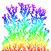
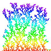
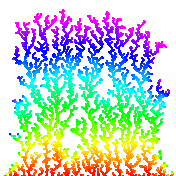
Program DLA.java simulates the growth of a DLA with the following properties. It uses the helper data type Picture.java. Set the initial aggregate to be the bottom row of the N-by-N lattice. Launch the particles from a random cell in top row. Assume that the particle goes up with probability 0.15, down with probability 0.35, and left or right with probability 1/4 each. Continue until the particles stick to a neighboring cell (above, below, left, right, or one of the four diagonals) or leaves the N-by-N lattice. The preferred downward direction is analogous to the effect of a temperature gradient on Brownian motion, or like how when a crystal is formed, the bottom of the aggregate is cooled more than the top; or like the influence of a gravitational force. For effect, we color the particles in the order they are released according to the rainbow from red to violet. Below are three simulations with N = 176; here is an image with N = 600.

Brownian motion. Brownian motion is a random process used to model a wide variety of physical phenomenon including the dispersion of ink flowing in water, and the behavior of atomic particles predicted by quantum physics. (more applications). Fundamental random process in the universe. It is the limit of a discrete random walk and the stochastic analog of the Gaussian distribution. It is now widely used in computational finance, economics, queuing theory, engineering, robotics, medical imaging, biology, and flexible manufacturing systems. First studied by a Scottish botanist Robert Brown in 1828 and analyzed mathematically by Albert Einstein in 1905. Jean-Baptiste Perrin performed experiments to confirm Einstein's predictions and won a Nobel Prize for his work. An applet to illustrate physical process that may govern cause of Brownian motion.

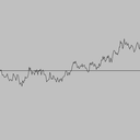
Simulating a Brownian motion. Since Brownian motion is a continuous and stochastic process, we can only hope to plot one path on a finite interval, sampled at a finite number of points. We can interpolate linearly between these points (i.e., connect the dots). For simplicitly, we'll assume the interval is from 0 to 1 and the sample points t₀, t₁, ..., t_N are equally spaced in this interval. To simulate a standard Brownian motion, repeatedly generate independent Gaussian random variables with mean 0 and standard deviation sqrt(1/N). The value of the Brownian motion at time i is the sum of the first i increments.

Geometric Brownian motion. A variant of Brownian motion is widely used to model stock prices, and the Nobel-prize winning Black-Scholes model is centered on this stochastic process. A geometric Brownian motion with drift μ and volatility σ is a stochastic process that can model the price of a stock. The parameter μ models the percentage drift. If μ = 0.10, then we expect the stock to increase by 10% each year. The parameter σ models the percentage volatility. If σ = 0.20, then the standard deviation of the stock price over one year is roughly 20% of the current stock price. To simulate a geometric Brownian motion from time t = 0 to t = T, we follow the same procedure for standard Brownian motion, but multiply the increments, instead of adding them, and incorporate the drift and volatility parameters. Specifically, we multiply the current price by by (1 + μΔt + σsqrt(Δt)Z), where Z is a standard Gaussian and Δt = T/N Start with X(0) = 100, σ = 0.04.

construction of BM.

Black-Scholes formula. Move to here?

Ising model. The motions of electrons around a nucleus produce a magnetic field associated with the atom. These atomic magnets act much like conventional magnets. Typically, the magnets point in random directions, and all of the forces cancel out leaving no overall magnetic field in a macroscopic clump of matter. However, in some materials (e.g., iron), the magnets can line up producing a measurable magnetic field. A major achievement of 19th century physics was to describe and understand the equations governing atomic magnets. The probability that state S occurs is given by the Boltzmann probability density function P(S) = e^-E(S)/kT / Z, where Z is the normalizing constant (partition function) sum e^-E(A)/kT over all states A, k is Boltzmann's constant, T is the absolute temperature (in degrees Kelvin), and E(S) is the energy of the system in state S.

Ising model proposed to describe magnetism in crystalline materials. Also models other naturally occurring phenomena including: freezing and evaporation of liquids, protein folding, and behavior of glassy substances.

Ising model. The Boltzmann probability function is an elegant model of magnetism. However, it is not practical to apply it for calculating the magnetic properties of a real iron magnet because any macroscopic chunk of iron contains an enormous number atoms and they interact in complicated ways. The Ising model is a simplified model for magnets that captures many of their important properties, including phase transitions at a critical temperature. (Above this temperature, no macroscopic magnetism, below it, systems exhibits magnetism. For example, iron loses its magnetization around 770 degrees Celsius. Remarkable thing is that transition is sudden.) reference

First introduced by Lenz and Ising in the 1920s. In the Ising model, the iron magnet is divided into an N-by-N grid of cells. (Vertex = atom in crystal, edge = bond between adjacent atoms.) Each cell contains an abstract entity known as spin. The spin s_i of cell i is in one of two states: pointing up (+1) or pointing down (-1). The interactions between cells is limited to nearest neighbors. The total magnetism of the system M = sum of s_i. The total energy of the system E = sum of - J s_i s_j, where the sum is taken over all nearest neighbors i and j. The constant J measures the strength of the spin-spin interactions (in units of energy, say ergs). [The model can be extended to allow interaction with an external magnetic field, in which case we add the term -B sum of s_k over all sites k.] If J > 0, the energy is minimized when the spins are aligned (both +1 or both -1) - this models ferromagnetism. if J < 0, the energy is minimized when the spins are oppositely aligned - this models antiferromagnetism.

Given this model, a classic problem in statistical mechanics is to compute the expected magenetism. A state is the specification of the spin for each of the N^2 lattice cells. The expected magnetism of the system E[M] = sum of M(S) P(S) over all states S, where M(S) is the magnetism of state S, and P(S) is the probability of state S occurring according to the Boltzmann probability function. Unfortunately, this equation is not amenable to a direct computational because the number of states S is 2^N*N for an N-by-N lattice. Straightforward Monte Carlo integration won't work because random points will not contribute much to sum. Need selective sampling, ideally sample points proportional to e^-E/kT. (In 1925, Ising solved the problem in one dimension - no phase transition. In a 1944 tour de force, Onsager solved the 2D Ising problem exactly. His solution showed that it has a phase transition. Not likely to be solved in 3D - see intractability section.)

Metropolis algorithm. Widespread usage of Monte Carlo methods began with Metropolis algorithm for calculation of rigid-sphere system. Published in 1953 after dinner conversation between Metropolis, Rosenbluth, Rosenbluth, Teller, and Teller. Widely used to study equilibrium properties of a system of atoms. Sample using Markov chain using Metropolis' rule: transition from A to B with probability 1 if Δ E <= 0, and with probability e^-ΔE/kT if Δ E > 0. When applied to the Ising model, this Markov chain is ergodic (similar to Google PageRank requirement) so the theory underlying the Metropolis algorithm applies. Converges to stationary distribution.

Program Cell.java, State.java, and Metropolis.java implements the Metropolis algorithm for a 2D lattice. Ising.java is a procedural programming version. "Doing physics by tossing dice." Simulate complicated physical system by a sequence of simple random steps.

Measuring physical quantities. Measure magnetism, energy, specific heat when system has thermalized (the system has reached a thermal equilibrium with its surrounding environment at a common temperature T). Compute the average energy and the average magenetization over time. Also interesting to compute the variance of the energy or specific heat <c> = <E²> - <E>², and the variance of the magnetization or susceptibility <Χ> = <M²> - <M>². Determining when system has thermalized is a challenging problem - in practice, many scientists use ad hoc methods.

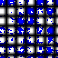
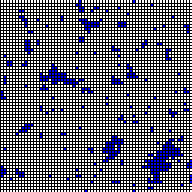
Phase transition. Phase transition occurs when temperature T_c is 2 / ln(1 + sqrt(2)) = 2.26918). T_c is known as the Curie temperature. Plot magnetization M (average of all spins) vs. temperature (kT = 1 to 4). Discontinuity of slope is signature of second order phase transition. Slope approaches infinity. Plot energy (average of all spin-spin interactions) vs. temperature (kT = 1 to 4). Smooth curve through phase transition. Compare against exact solution. Critical temperature for which algorithm dramatically slows down. Below are the 5000th sample trajectory for J/kT = 0.4 (hot / disorder) and 0.47 (cold / order). The system becomes magnetic as temperature decreases; moreover, as temperature decreases the probability that neighboring sites have the same spin increasing (more clumping).

Experiments.

Start will above critical temperature. State converges to nearly uniform regardless of initial state (all up, all down, random) and fluctuates rapidly. Zero magnetization.
Start well below critical temperature. Start all spins with equal value (all up or all down). A few small clusters of opposite spin form.
Start well below critical temperature. Start with random spins. Large clusters of each spin form; eventually simulation makes up its mind. Equally likely to have large clusters in up or down spin.
Start close to critical temperature. Large clusters form, but fluctuate very slowly.

Exact solution for Ising model known for 1D and 2D; NP-hard for 3d and nonplanar graphs.

Models phase changes in binary alloys and spin glasses. Also models neural networks, flocking birds, and beating heart cells. Over 10,000+ papers published using the Ising model.

Q + A

Exercises

Print a random word. Read in a list of words (of unknown length) from standard input, and print out one of the N words uniformly at random. Do not store the word list. Instead, use Knuth's method: when reading in the ith word, select it with probability 1/i to be the new champion. Print out the word that survives after reading in all of the data.
Random subset of a linked list. Given an array of N elements and an integer k ≤ N, construct a new array containing a random subset of k elements. Hint: traverse the array, either accepting each element with probability a/b, where a is the number of elements left to select, and b is the number of elements remaining.

Creative Exercises

Random number generation. Can the following for computing a pseudo-random integer between 0 and N-1 fail? Math.random is guaranteed to return a floating point number greater than or equal to 0.0 and strictly less than 1.0.
double x = Math.random(); int r = (int) (x * N);
That is, can you find a real number x and an integer N for which r equals N?

Solution: No, it can't happen in IEEE floating point arithmetic. The roundoff error will not cause the result to be N, even if Math.random returns 0.9999999999.... However, this method does not produce integers uniformly at random because floating point numbers are not evenly distributed. Also, it involves casting and multiplying, which are excessive.
Random number test. Write a program to plot the outcome of a boolean pseudo-random number generator. For simplicity, use (Math.random() < 0.5) and plot in a 128-by-128 grid like the following pseudorandom applet. Perhaps use LFSR or Random.nextLong() % 2.
Sampling from a discrete probability distribution. Suppose that there are N events and event i occurs with probability p_i, where p₀ + p₁ + ... + p_N-1 = 1. Write a program Sample.java that prints out 1,000 sample events according to the probability distribution. Hint: choose a random number r between 0 and 1 and iterate from i = 0 to N-1 until p₀ + p₁ + ... + p_i > r. (Be careful about floating point precision.)
Sampling from a discrete probability distribution. Improve the algorithm from the previous problem so that it takes time proportional to log N to generate a new sample. Hint: binary search on the cumulative sums. Note: see this paper for a very clever alternative that generates random samples in a constant amount of time. Discrete.java is a Java version of Warren D. Smith's WDSsampler.c program.
Sampling from a discrete probability distribution. Repeat the previous question but make it dynamic. That is, after each sample, the probabilities of some events might change, or there may be new events. Used in n-fold way algorithm, which is method of choice for kinetic Monte Carlo methods where one wants to simulate the kinetic evolution process. Typical application: simulating gas reacting with surface of a substrate where chemical reaction occur at different rates. Hint: use a binary search tree.
Zipf distribution. Use the result of the previous exercise(s) to sample from the Zipfian distribution with parameter s and N. The distribution can take on integer values from 1 to N, and takes on value k with probability 1/k^s / sum_(i = 1 to N) 1/i^s. Example: words in Shakespeare's play Hamlet with s approximately equal to 1.
Simulating a Markov chain. Write a program MarkovChain.java that simulates a Markov chain. Hint: you will need to sample from a discrete distribution.
DLA with non-unity sticking probability Modify DLA.java so that the initial aggregate consists of several randomly spaced cells along the bottom of the lattice. This simulates string-like bacterial growth.
DLA with non-unity sticking probability Modify DLA.java to allow a sticking probability less than one. That is, if a particle has a neighbor, then it sticks with probability p < 1.0; otherwise, it moves at random to a neighboring cell which is unoccupied. This results in a gives more clustered structure, simulating higher bond affinity between atoms.
Symmetric DLA. Initialize the aggregate to be a single particle in the center of the lattice. Launch particles uniformly from a circle centered at the initial particle. Increase the size of the launch circle as the size of the aggregate increases. Name your program SymmetricDLA.java. This simulates the growth of an aggregate where the particles wander in randomly from infinity. Here are some tricks for speeding up the process.
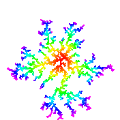
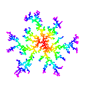
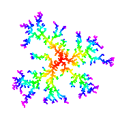
Variable sticking probability. A wandering particle which enters an empty site next to an occupied site is assigned a random number, indicating a potential direction in which the particle can move (up, down, left or right). If an occupied site exists on the new site indicated by the random number, then the particle sticks to the aggregate by occupying its current lattice site. If not, it moves to that site and the random walk continues. This simulates snowflake growth.
Random walk solution of Laplace's equation. Numerically solve Laplace's equation to determine the electric potential given the positions of the charges on the boundary. Laplace's equation says that the gradient of the potential is the sum of the second partial derivatives with respect to x and y. See Gould and Tobochnik, 10.2. Your goal is to find the function V(x, y) that satisfies Laplace's equation at specified boundary conditions. Assume the charge-free region is a square and that the potential is 10 along the vertical boundaries and 5 along the horizontal ones. To solve Laplace's equation, divide the square up into an N-by-N grid of points. The potential V(x, y) of cell (x, y) is the average of the potentials at the four neighboring cells. To estimate V(x, y), simulate 1 million random walkers starting at cell (x, y) and continuing until they reach the boundary. An estimate of V(x, y) is the average potential at the 1 million boundary cells reached. Write a program Laplace.java that takes three command line parameters N, x, and y and estimates V(x, y) over an N-by-N grid of cells where the potential at column 0 and N is 10 and the potential at row 0 and N is 5.Remark: although the boundary value problem above can be solved analytically, numerical simulations like the one above are useful when the region has a more complicated shape or needs to be repeated for different boundary conditions.
simulated annealing
Simulating a geometric random variable. If some event occurs with probability p, a geometric random variable with parameter p models the number N of independent trials needed between occurrence of the event. To generate a variable with the geometric distribution, use the following formula

N = ceil(ln U / ln (1 - p))

where U is a variable with the uniform distribution. Use the Math library methods Math.ceil, Math.log, and Math.random.
Simulating an exponential random variable. The exponential distribution is widely used to model the the inter-arrival time between city buses, the time between failure of light bulbs, etc. The probability that an exponential random variable with parameter λ is less than x is F(x) = 1 - e^{λ x} for x >= 0. To generate a random deviate from the distribution, use the inverse function method: output -ln(U) / λ where U is a uniform random number between 0 and 1.

Poisson distribution. The Poisson distribution is useful in describing the fluctuations in the number of nuclei that decay in any particular small time interval.

public static int poisson(double c) {
   double t = 0.0;
   for (int x = 0; true; x++) {
      t = t - Math.log(Math.random()) / c;  // sum exponential deviates
      if (t > 1.0) return x;
   }
}

Simulating a Pareto random variable. The Pareto distribution is often used to model insurance claims damages, financial option holding times, and Internet traffic activity. The probability that a Pareto random variable with parameter a is less than x is F(x) = 1 - (1 + x)^-a for x >= 0. To generate a random deviate from the distribution, use the inverse function method: output (1-U)^-1/a - 1, where U is a uniform random number between 0 and 1.
Simulating a Cauchy random variable. The density function of a Cauchy random variable is f(x) = 1/(Π(1 + x²)). The probability that a Cauchy random variable is less than x is F(x) = 1/Π (Π/2 + arctan(x)). To generate a random deviate from the distribution, use the inverse function method: output tan(Π(U - 1/2)), where U is a uniform random number between 0 and 1.
Generate random point inside unit disc. Incorrect to choose set r uniformly between 0 and 1, θ uniformly between 0.0 and 2π, and use (x, y) = (r cosθ, r sinθ). If you do this, more points close to center of disc. Instead, set (x, y) = (√r cos&theta, √r sinθ) Alternatively, generate x and y uniformly between -1 and 1 and accept if x² + y² ≤ 1. Plot a random sequence of points using both methods and see the bias.
Flipping bits. As part of a genetic algorithm, suppose you need to flip N bits independently, each with probability p, where p is some very small constant.
- Method 1: loop through N bits, generate a Bernouilli(p) random variable for each one and flip accordingly. Takes time proportional to N.
- Method 2: generate a Geometric(p) random variable X_0 and flip bit X_0; genereate another Geometric(p) random variable an flip bit X_0 + X_1, and so on. Takes time proportional to Np.
- Method 3: the number of bits to flip in Binomial(N, p). Determine how many bits to flip by approximating with a Gaussian(Np, sigma) random variable. Then flip Z bits, taking care not to avoid duplicates. Takes time proportional to Np, but less calls to transcendental functions.
Random point inside N-dimensional sphere. Write a program InsideSphere.java that takes a command line parameter N and computes a random point inside an N-dimensional sphere with radius 1. Generate N uniform random variables deviates x₁, ..., x_N and use this point if
(x₁)² + ... + (x_N)² ≤ 1
Otherwise repeat.
Random point on surface of an N-dimensional sphere. Write a program Sphere.java that takes a command line parameter N and computes a random point on the surface of an N-dimensional sphere with radius 1 using Brown's method. Brown's method is to compute N independent standard normal deviates x₁, x_N. Then
( x₁/r, x₂/r, ..., x_N/r ), where r = sqrt((x₁)² + ... + (x_N)²)
has the desired distribution. Use Exercise xyz from Section 3 to compute standard normal deviates.
Potts model. The Potts model is a variant of the Ising model where each site has q possible directions. (q = 2 corresponds to Ising) The total energy of the system E = sum of - J sigma(s_i, s_j) over all neighbors. The Kronecker delta function δ(x, y) = 1 if x = y and 0 otherwise.
2D Brownian motion. Simulate diffusion of particles in a fluid. Write a data type BrownianParticle.java that represents a particle undergoing a Brownian motion in two dimensions. To do this, simulate two indepedent Brownian motions X(t) and Y(t), and plot (X(t), Y(t)). Create a client program that takes a command line integer N, creates N particles at the origin, and simulates a Brownian motion for the N particles.
Brownian bridge. A Browian bridge is a constratined Brownian motion, which is required to begin at the origin at time 0, and end at the origin at time T. If X(t) is a Brownian motion then Z(t) = X(t) - (t/T)X(T) is such a process. To plot, store the intermediate values X(t) and plot after you've computed X(T).
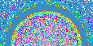
Rainbow. In 1637 Rene Descartes discovered the first scientific explanation for the formation of rainbows. His method involved tracing the internal reflections when a light ray is sent through a a spherical raindrop. Simulate the generation of a rainbow according to model of large number of parallel rays hitting a spherical raindrop. When a light ray hit a raindrop, the ray is reflected and refracted. We use the HSB color format, and choose the hue h at random between 0 (red) and 1 (violet). We use 1.33 + 0.06 * h for the refraction index of hue h. For each ray, we plot a single point of light, according to physical laws of refraction and reflection. Each point of light is then plotted in a random color that the observer will see, either in the primary or secondary rainbow. To perform the simulation, we choose one of the 7 colors uniformly at random. Then, we choose a point (x, y) in the unit circle, centered at (0, 0) and set the impact parameter r = sqrt(x² + y²). The angle of incidence θ_i = arcsin(r) and, by Snell's law, the angle of refraction θ_r = arcsin (r / n), where n is the refraction index. If the light ray is totally reflected only once, it emerges at an angle of θ_p = 4θ_r - 2θ_i, contributing to the primary rainbow. If the light ray is totally reflected a second time, it emerges at an angle of θ_p = 6θ_r - 2θ_i - π, contributing to the secondary rainbow. The intensities I_p and I_s of the primary and secondary rays are calculated according to the following transmission and reflection formulas for electromagnetic waves across the boundary of two media.
I_p = 1/2 (s(1-s)² + p(1-p)²) I_s = 1/2 (s²(1-s)² + p²(1-p)²) p = (sin(θ_i-θ_r)/sin(θ_i+θ_r))² r = (tan(θ_i-θ_r)/tan(θ_i+θ_r))²
The color intensities I_p and I_s are used to determine the saturation in the HSB color format. Program Rainbow.java simulates this process.

Rainbow site.

Last modified on January 31, 2009.

Copyright © 2000–2019 Robert Sedgewick and Kevin Wayne. All rights reserved.

thetechnodepot.com