https://github.com/kevin-wayne/algs4/tree/master/src/main/java/edu/princeton/cs/algs4
COS 126 Java Programming
https://introcs.cs.princeton.edu/java/code/
Java Programs in the Textbook
Standard libraries.
Here are the standard input and output libraries that we use throughout the textbook.
Programs in the textbook.
Below is a table of the Java programs in the textbook. Click on the program name to access the Java code; click on the reference number for a brief description; read the textbook for a full discussion. You can download all of the programs as introcs.jar and the data as introcs-data.zip; you can also download all of the programs and data as the IntelliJ project IntroCS.zip.
| 1 | ELEMENTS OF PROGRAMMING | |
|---|---|---|
| 1.1.1 | HelloWorld.java | Hello, World |
| 1.1.2 | UseArgument.java | using a command-line argument |
| 1.2.1 | Ruler.java | string concatenation example |
| 1.2.2 | IntOps.java | integer multiplication and division |
| 1.2.3 | Quadratic.java | quadratic formula |
| 1.2.4 | LeapYear.java | leap year |
| 1.2.5 | RandomInt.java | casting to get a random integer |
| 1.3.1 | Flip.java | flippling a fair coin |
| 1.3.2 | TenHellos.java | your first while loop |
| 1.3.3 | PowersOfTwo.java | computing powers of 2 |
| 1.3.4 | DivisorPattern.java | your first nested loops |
| 1.3.5 | HarmonicNumber.java | harmonic numbers |
| 1.3.6 | Sqrt.java | Newton's method |
| 1.3.7 | Binary.java | converting to binary |
| 1.3.8 | Gambler.java | gambler's ruin simulation |
| 1.3.9 | Factors.java | factoring integers |
| 1.4.1 | Sample.java | sampling without replacement |
| 1.4.2 | CouponCollector.java | coupon collector simulation |
| 1.4.3 | PrimeSieve.java | sieve of Eratosthenes |
| 1.4.4 | SelfAvoidingWalk.java | self-avoiding random walks |
| 1.5.1 | RandomSeq.java | generating a random sequence |
| 1.5.2 | TwentyQuestions.java | interactive user input |
| 1.5.3 | Average.java | averaging a stream of numbers |
| 1.5.4 | RangeFilter.java | a simple filter |
| 1.5.5 | PlotFilter.java | standard input-to-drawing filter |
| 1.5.6 | BouncingBall.java | bouncing ball |
| 1.5.7 | PlayThatTune.java | digital signal processing |
| 1.6.1 | Transition.java | computing the transition matrix |
| 1.6.2 | RandomSurfer.java | simulating a random surfer |
| 1.6.3 | Markov.java | mixing a Markov chain |
| 2 | FUNCTIONS | |
| 2.1.1 | Harmonic.java | harmonic numbers (revisited) |
| 2.1.2 | Gaussian.java | Gaussian functions |
| 2.1.3 | Coupon.java | coupon collector (revisited) |
| 2.1.4 | PlayThatTuneDeluxe.java | play that tune (revisited) |
| 2.2.1 | StdRandom.java | random number library |
| 2.2.2 | StdArrayIO.java | array I/O library |
| 2.2.3 | IFS.java | iterated function systems |
| 2.2.4 | StdStats.java | data analysis library |
| 2.2.5 | StdStats.java | data analysis library |
| 2.2.6 | Bernoulli.java | Bernoulli trials |
| 2.3.1 | Euclid.java | Euclid's algorithm |
| 2.3.2 | TowersOfHanoi.java | towers of Hanoi |
| 2.3.3 | Beckett.java | Gray code |
| 2.3.4 | Htree.java | recursive graphics |
| 2.3.5 | Brownian.java | Brownian bridge |
| 2.3.6 | LongestCommonSubsequence.java | longest common subsequence |
| 2.4.1 | Percolation.java | percolation scaffolding |
| 2.4.2 | VerticalPercolation.java | vertical percolation |
| 2.4.3 | PercolationVisualizer.java | percolation visualization client |
| 2.4.4 | PercolationProbability.java | percolation probability estimate |
| 2.4.5 | Percolation.java | percolation detection |
| 2.4.6 | PercolationPlot.java | adaptive plot client |
| 3 | OBJECT ORIENTED PROGRAMMING | |
| 3.1.1 | PotentialGene.java | identifying a potential gene |
| 3.1.2 | AlbersSquares.java | Albers squares |
| 3.1.3 | Luminance.java | luminance library |
| 3.1.4 | Grayscale.java | converting color to grayscale |
| 3.1.5 | Scale.java | image scaling |
| 3.1.6 | Fade.java | fade effect |
| 3.1.7 | Cat.java | concatenating files |
| 3.1.8 | StockQuote.java | screen scraping for stock quotes |
| 3.1.9 | Split.java | splitting a file |
| 3.2.1 | Charge.java | charged-particle data type |
| 3.2.2 | Stopwatch.java | stopwatch data type |
| 3.2.3 | Histogram.java | histogram data type |
| 3.2.4 | Turtle.java | turtle graphics data type |
| 3.2.5 | Spiral.java | spira mirabilis |
| 3.2.6 | Complex.java | complex number data type |
| 3.2.7 | Mandelbrot.java | Mandelbrot set |
| 3.2.8 | StockAccount.java | stock account data type |
| 3.3.1 | Complex.java | complex number data type (revisited) |
| 3.3.2 | Counter.java | counter data type |
| 3.3.3 | Vector.java | spatial vector data type |
| 3.3.4 | Sketch.java | document sketch data type |
| 3.3.5 | CompareDocuments.java | similarity detection |
| 3.4.1 | Body.java | gravitational body data type |
| 3.4.2 | Universe.java | n-body simulation |
| 4 | DATA STRUCTURES | |
| 4.1.1 | ThreeSum.java | 3-sum problem |
| 4.1.2 | DoublingTest.java | validating a doubling hypothesis |
| 4.2.1 | Questions.java | binary search (20 questions) |
| 4.2.2 | Gaussian.java | bisection search |
| 4.2.3 | BinarySearch.java | binary search (in a sorted array) |
| 4.2.4 | Insertion.java | insertion sort |
| 4.2.5 | InsertionTest.java | doubling test for insertion sort |
| 4.2.6 | Merge.java | mergesort |
| 4.2.7 | FrequencyCount.java | frequency counts |
| 4.3.1 | ArrayStackOfStrings.java | stack of strings (array) |
| 4.3.2 | LinkedStackOfStrings.java | stack of strings (linked list) |
| 4.3.3 | ResizingArrayStackOfStrings.java | stack of strings (resizing array) |
| 4.3.4 | Stack.java | generic stack |
| 4.3.5 | Evaluate.java | expression evaluation |
| 4.3.6 | Queue.java | generic queue |
| 4.3.7 | MM1Queue.java | M/M/1 queue simulation |
| 4.3.8 | LoadBalance.java | load balancing simulation |
| 4.4.1 | Lookup.java | dictionary lookup |
| 4.4.2 | Index.java | indexing |
| 4.4.3 | HashST.java | hash table |
| 4.4.4 | BST.java | binary search tree |
| 4.4.5 | DeDup.java | dedup filter |
| – | ST.java | symbol table data type |
| – | SET.java | set data type |
| 4.5.1 | Graph.java | graph data type |
| 4.5.2 | IndexGraph.java | using a graph to invert an index |
| 4.5.3 | PathFinder.java | shortest-paths client |
| 4.5.4 | PathFinder.java | shortest-paths implementation |
| 4.5.5 | SmallWorld.java | small-world test |
| 4.5.6 | Performer.java | performer–performer graph |
Exercise solutions.
Here is a list of solutions to selected coding exercises.
| 1 | ELEMENTS OF PROGRAMMING | |
|---|---|---|
| 1.1.1 | TenHelloWorlds.java | ten Hello, Worlds |
| 1.1.5 | UseThree.java | three command-line arguments |
| 1.2.20 | SumOfTwoDice.java | sum of two dice |
| 1.2.23 | SpringSeason.java | is month and day in Spring? |
| 1.2.25 | WindChill.java | compute wind chill factor |
| 1.2.26 | CartesianToPolar.java | Cartesian to polar coordinates |
| 1.2.29 | DayOfWeek.java | compute day of week from date |
| 1.2.30 | Stats5.java | average, min, max of 5 random numbers |
| 1.2.34 | ThreeSort.java | sort three integers |
| 1.2.35 | Dragon.java | dragon curve of order 5 |
| 1.3.8 | FivePerLine.java | print integers five per line |
| 1.3.11 | FunctionGrowth.java | table of functions |
| 1.3.12 | DigitReverser.java | reverse digits |
| 1.3.13 | Fibonacci.java | Fibonacci numbers |
| 1.3.15 | SeriesSum.java | convergent sum |
| 1.3.31 | Ramanujan.java | taxicab numbers |
| 1.3.32 | ISBN.java | ISBN checksum |
| 1.3.38 | Sin.java | sine function via Taylor series |
| 1.3.41 | MonteHall.java | Monte Hall problem |
| 1.4.2 | HugeArray.java | creating a huge array |
| 1.4.10 | Deal.java | deal poker hands |
| 1.4.13 | Transpose.java | tranpose a square matrix |
| 1.4.25 | InversePermutation.java | compute inverse permutation |
| 1.4.26 | Hadamard.java | compute Hadamard matrix |
| 1.4.30 | Minesweeper.java | create Minesweeper board |
| 1.4.33 | RandomWalkers.java | N random walkers |
| 1.4.35 | Birthdays.java | birthday problem |
| 1.4.37 | BinomialCoefficients.java | binomial coefficients |
| 1.5.1 | MaxMin.java | max and min from standard input |
| 1.5.3 | Stats.java | mean and stddev from standard input |
| 1.5.5 | LongestRun.java | longest consecutive run from stdin |
| 1.5.11 | WordCount.java | word count from standard input |
| 1.5.15 | Closest.java | closest point |
| 1.5.18 | Checkerboard.java | draw a checkerboard |
| 1.5.21 | Rose.java | draw a rose |
| 1.5.22 | Banner.java | animate a text banner |
| 1.5.31 | Spirograph.java | draw spirograph |
| 1.5.32 | Clock.java | animate a clock |
| 1.5.33 | Oscilloscope.java | simulate an oscilloscope |
| 2 | FUNCTIONS | |
| 2.1.4 | ArrayEquals.java | are two integer arrays equal? |
| 2.1.30 | BlackScholes.java | Black-Scholes option valuation |
| 2.1.32 | Horner.java | Horner's method to evaluate a polynomial |
| 2.1.33 | Benford.java | Benford's law |
| 2.1.38 | Calendar.java | create a calendar |
| 2.2.1 | Gaussian.java | overloaded gaussian distribution functions |
| 2.2.2 | Hyperbolic.java | hyperbolic trig functions |
| 2.2.4 | StdRandom.java | shuffle an array of doubles |
| 2.2.6 | StdArrayIO.java | array IO methods |
| 2.2.11 | Matrix.java | matrix operations |
| 2.2.12 | MarkovSquaring.java | page rank via matrix squaring |
| 2.2.14 | StdRandom.java | exponential random variable |
| 2.3.14 | AnimatedHtree.java | animated H-tree |
| 2.3.15 | IntegerToBinary.java | integer to binary conversion |
| 2.3.17 | Permutations.java | all permutations |
| 2.3.18 | PermutationsK.java | all permutations of size k |
| 2.3.19 | Combinations.java | all combinations |
| 2.3.20 | CombinationsK.java | all combinations of size k |
| 2.3.22 | RecursiveSquares.java | recursive squares |
| 2.3.24 | GrayCode.java | Gray code |
| 2.3.26 | AnimatedHanoi.java | animated Towers of Hanoi |
| 2.3.29 | Collatz.java | Collatz function |
| 2.3.30 | BrownianIsland.java | Brownian island |
| 2.3.31 | PlasmaCloud.java | plama cloud |
| 2.3.32 | McCarthy.java | McCarthy's 91 function |
| 2.3.33 | Tree.java | fractal tree |
| 2.4.15 | PercolationDirectedNonrecursive.java | directed percolation |
Copyright © 2000–2019 Robert Sedgewick and Kevin Wayne. All rights reserved.
COS 126 Python Language
Python Programs in the Textbook
Booksite Modules
Below is a table of the booksite modules that we use throughout the textbook and booksite and beyond.
| SECTION | MODULE | DESCRIPTION |
|---|---|---|
| 1.5 | stdio.py | functions to read/write numbers and text from/to stdin and stdout |
| 1.5 | stddraw.py | functions to draw geometric shapes |
| 1.5 | stdaudio.py | functions to create, play, and manipulate sound |
| 2.2 | stdrandom.py | functions related to random numbers |
| 2.2 | stdarray.py | functions to create, read, and write 1D and 2D arrays |
| 2.2 | stdstats.py | functions to compute and plot statistics |
| 3.1 | color.py | data type for colors |
| 3.1 | picture.py | data type to process digital images |
| 3.1 | instream.py | data type to read numbers and text from files and URLs |
| 3.1 | outstream.py | data type to write numbers and text to files |
If you followed the instructions provided in this booksite (for Windows, Mac OS X, or Linux), then the booksite modules are installed on your computer. If you want to see the source code for the booksite modules, then click on the links in the above table, or download and unzip stdlib-python.zip.
Programs and Data Sets in the Textbook
Below is a table of the Python programs and data sets used in the textbook. Click on the program name to access the Python code; click on the data set name to access the data set; read the textbook for a full discussion. You can download all of the programs as introcs-python.zip and the data as introcs-data.zip.
| 1 | ELEMENTS OF PROGRAMMING | DATA | |
|---|---|---|---|
| 1.1.1 | helloworld.py | Hello, World | – |
| 1.1.2 | useargument.py | using a command-line argument | – |
| 1.2.1 | ruler.py | string concatenation example | – |
| 1.2.2 | intops.py | integer operators | – |
| 1.2.3 | floatops.py | float operators | – |
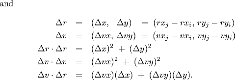
| 1.2.4 | quadratic.py | quadratic formula | – |
| 1.2.5 | leapyear.py | leap year | – |
| 1.3.1 | flip.py | flipping a fair coin | – |
| 1.3.2 | tenhellos.py | your first loop | – |
| 1.3.3 | powersoftwo.py | computing powers of two | – |
| 1.3.4 | divisorpattern.py | your first nested loops | – |
| 1.3.5 | harmonic.py | harmonic numbers | – |
| 1.3.6 | sqrt.py | Newton's method | – |
| 1.3.7 | binary.py | converting to binary | – |
| 1.3.8 | gambler.py | gambler's ruin simulation | – |
| 1.3.9 | factors.py | factoring integers | – |
| 1.4.1 | sample.py | sampling without replacement | – |
| 1.4.2 | couponcollector.py | coupon collector simulation | – |
| 1.4.3 | primesieve.py | sieve of Eratosthenes | – |
| 1.4.4 | selfavoid.py | self-avoiding random walks | – |
| 1.5.1 | randomseq.py | generating a random sequence | – |
| 1.5.2 | twentyquestions.py | interactive user input | – |
| 1.5.3 | average.py | averaging a stream of numbers | – |
| 1.5.4 | rangefilter.py | a simple filter | – |
| 1.5.5 | plotfilter.py | standard input to draw filter | usa.txt |
| 1.5.6 | bouncingball.py | bouncing ball | – |
| 1.5.7 | playthattune.py | digital signal processing | elise.txt ascale.txt stairwaytoheaven.txt entertainer.txt firstcut.txt freebird.txt looney.txt |
| 1.6.1 | transition.py | computing the transition matrix | small.txt medium.txt |
| 1.6.2 | randomsurfer.py | simulating a random surfer | – |
| 1.6.3 | markov.py | mixing a Markov chain | – |
| 2 | FUNCTIONS | DATA | |
| 2.1.1 | harmonicf.py | harmonic numbers (revisited) | – |
| 2.1.2 | gauss.py | Gaussian functions | – |
| 2.1.3 | coupon.py | coupon collector (revisited) | – |
| 2.1.4 | playthattunedeluxe.py | play that tune (revisited) | elise.txt ascale.txt stairwaytoheaven.txt entertainer.txt firstcut.txt freebird.txt looney.txt |
| 2.2.1 | gaussian.py | Gaussian functions module | – |
| 2.2.2 | gaussiantable.py | sample Gaussian client | – |
| 2.2.3 | sierpinski.py | Sierpinski triangle | – |
| 2.2.4 | ifs.py | iterated function systems | sierpinski.txt barnsley.txt coral.txt culcita.txt cyclosorus.txt dragon.txt fishbone.txt floor.txt koch.txt spiral.txt swirl.txt tree.txt zigzag.txt |
| 2.2.5 | bernoulli.py | Bernoulli trials | – |
| 2.3.1 | euclid.py | Euclid's algorithm | – |
| 2.3.2 | towersofhanoi.py | towers of Hanoi | – |
| 2.3.3 | beckett.py | Gray code | – |
| 2.3.4 | htree.py | recursive graphics | – |
| 2.3.5 | brownian.py | Brownian bridge | – |
| 2.4.1 | percolationv.py | vertical percolation detection | test5.txt test8.txt |
| 2.4.2 | percolationio.py | percolation support functions | – |
| 2.4.3 | visualizev.py | vertical percolation visualization client | – |
| 2.4.4 | estimatev.py | vertical percolation probability estimate | – |
| 2.4.5 | percolation.py | percolation detection | test5.txt test8.txt |
| 2.4.6 | visualize.py | percolation visualization client | – |
| 2.4.7 | estimate.py | percolation probability estimate | – |
| 3 | OBJECT ORIENTED PROGRAMMING | DATA | |
| 3.1.1 | potentialgene.py | potential gene identification | – |
| 3.1.2 | chargeclient.py | charged particle client | – |
| 3.1.3 | alberssquares.py | Albers squares | – |
| 3.1.4 | luminance.py | luminance library | – |
| 3.1.5 | grayscale.py | converting color to grayscale | mandrill.jpg mandrill.png darwin.jpg darwin.png |
| 3.1.6 | scale.py | image scaling | mandrill.jpg mandrill.png darwin.jpg darwin.png |
| 3.1.7 | fade.py | fade effect | mandrill.jpg mandrill.png darwin.jpg darwin.png |
| 3.1.8 | potential.py | visualizing electric potential | charges.txt |
| 3.1.9 | cat.py | concatenating files | in1.txt in2.txt |
| 3.1.10 | stockquote.py | screen scraping for stock quotes | – |
| 3.1.11 | split.py | splitting a file | djia.csv |
| 3.2.1 | charge.py | charged-particle data type | – |
| 3.2.2 | stopwatch.py | stopwatch data type | – |
| 3.2.3 | histogram.py | histogram data type | – |
| 3.2.4 | turtle.py | turtle graphics data type | – |
| 3.2.5 | koch.py | Koch curve | – |
| 3.2.6 | spiral.py | spira mirabilis | – |
| 3.2.7 | drunk.py | drunken turtle | – |
| 3.2.8 | drunks.py | drunken turtles | – |
| 3.2.9 | complex.py | complex number data type | – |
| 3.2.10 | mandelbrot.py | Mandelbrot set | – |
| 3.2.11 | stockaccount.py | stock account data type | turing.txt |
| 3.3.1 | complexpolar.py | complex numbers (revisited) | – |
| 3.3.2 | counter.py | counter data type | – |
| 3.3.3 | vector.py | spatial vector data type | – |
| 3.3.4 | sketch.py | sketch data type | genome20.txt |
| 3.3.5 | comparedocuments.py | similarity detection | documents.txt constitution.txt tomsawyer.txt huckfinn.txt prejudice.txt djia.csv amazon.html actg.txt |
| 3.4.1 | body.py | gravitational body data type | – |
| 3.4.2 | universe.py | n-body simulation | 2body.txt 3body.txt 4body.txt 2bodytiny.txt |
| 4 | DATA STRUCTURES | DATA | |
| 4.1.1 | threesum.py | 3-sum problem | 8ints.txt 1kints.txt 2kints.txt 4kints.txt 8kints.txt 16kints.txt 32kints.txt 64kints.txt 128kints.txt |
| 4.1.2 | doublingtest.py | validating a doubling hypothesis | – |
| 4.1.3 | timeops.py | timing operators and functions | – |
| 4.1.4 | bigarray.py | discovering memory capacity | – |
| 4.2.1 | questions.py | binary search (20 questions) | – |
| 4.2.2 | bisection.py | binary search (inverting a function) | – |
| 4.2.3 | binarysearch.py | binary search (sorted array) | emails.txt white.txt |
| 4.2.4 | insertion.py | insertion sort | tiny.txt tomsawyer.txt |
| 4.2.5 | timesort.py | doubling test for sorting functions | – |
| 4.2.6 | merge.py | mergesort | tiny.txt tomsawyer.txt |
| 4.2.7 | frequencycount.py | frequency counts | leipzig100k.txt leipzig200k.txt leipzig1m.txt |
| 4.3.1 | arraystack.py | stack (resizing array implementation) | tobe.txt |
| 4.3.2 | linkedstack.py | stack (linked list implementation) | tobe.txt |
| 4.3.3 | evaluate.py | expression evaluation | expression1.txt expression2.txt |
| 4.3.4 | linkedqueue.py | queue (linked list implementation) | tobe.txt |
| 4.3.5 | mm1queue.py | M/M/1 queue simulation | – |
| 4.3.6 | loadbalance.py | load balancing simulation | – |
| 4.4.1 | lookup.py | dictionary lookup | amino.csv djia.csv elements.csv ip.csv ip-by-country.csv morse.csv phone-na.csv |
| 4.4.2 | index.py | indexing | mobydick.txt tale.txt |
| 4.4.3 | hashst.py | hash symbol table data type | – |
| 4.4.4 | bst.py | BST symbol table data type | – |
| 4.5.1 | graph.py | graph data type | tinygraph.txt |
| 4.5.2 | invert.py | using a graph to invert an index | tinygraph.txt movies.txt |
| 4.5.3 | separation.py | shortest-paths client | routes.txt movies.txt |
| 4.5.4 | pathfinder.py | shortest-paths client | – |
| 4.5.5 | smallworld.py | small-world test | tinygraph.txt |
| 4.5.6 | performer.py | performer-performer graph | tinymovies.txt moviesg.txt |
COS 126 Global Sequence Alignment
https://introcs.cs.princeton.edu/java/assignments/sequence.html
| COS 126
Global Sequence Alignment |
Programming Assignment |
Write a program to compute the optimal sequence alignment of two DNA strings. This program will introduce you to the emerging field of computational biology in which computers are used to do research on biological systems. Further, you will be introduced to a powerful algorithmic design paradigm known as dynamic programming.
Biology review. A genetic sequence is a string formed from a four-letter alphabet {Adenine (A), Thymine (T), Guanine (G), Cytosine (C)} of biological macromolecules referred to together as the DNA bases. A gene is a genetic sequence that contains the information needed to construct a protein. All of your genes taken together are referred to as the human genome, a blueprint for the parts needed to construct the proteins that form your cells. Each new cell produced by your body receives a copy of the genome. This copying process, as well as natural wear and tear, introduces a small number of changes into the sequences of many genes. Among the most common changes are the substitution of one base for another and the deletion of a substring of bases; such changes are generally referred to as point mutations. As a result of these point mutations, the same gene sequenced from closely related organisms will have slight differences.
The problem. Through your research you have found the following sequence of a gene in a previously unstudied organism.
A A C A G T T A C C
What is the function of the protein that this gene encodes? You could begin a series of uninformed experiments in the lab to determine what role this gene plays. However, there is a good chance that it is a variant of a known gene in a previously studied organism. Since biologists and computer scientists have laboriously determined (and published) the genetic sequence of many organisms (including humans), you would like to leverage this information to your advantage. We'll compare the above genetic sequence with one which has already been sequenced and whose function is well understood.
T A A G G T C A
If the two genetic sequences are similar enough, we might expect them to have similar functions. We would like a way to quantify "similar enough."
Edit-distance. In this assignment we will measure the similarity of two genetic sequences by their edit distance, a concept first introduced in the context of coding theory, but which is now widely used in spell checking, speech recognition, plagiarism detection, file revisioning, and computational linguistics. We align the two sequences, but we are permitted to insert gaps in either sequence (e.g., to make them have the same length). We pay a penalty for each gap that we insert and also for each pair of characters that mismatch in the final alignment. Intuitively, these penalties model the relative likeliness of point mutations arising from deletion/insertion and substitution. We produce a numerical score according to the following simple rule, which is widely used in biological applications:
Penalty Cost Per gap 2 Per mismatch 1 Per match 0
As an example, two possible alignments of AACAGTTACC and TAAGGTCA are:
Sequence 1 A A C A G T T A C C Sequence 2 T A A G G T C A - - Penalty 1 0 1 1 0 0 1 0 2 2
Sequence 1 A A C A G T T A C C Sequence 2 T A - A G G T - C A Penalty 1 0 2 0 0 1 0 2 0 1
The first alignment has a score of 8, while the second one has a score of 7. The edit-distance is the score of the best possible alignment between the two genetic sequences over all possible alignments. In this example, the second alignment is in fact optimal, so the edit-distance between the two strings is 7. Computing the edit-distance is a nontrivial computational problem because we must find the best alignment among exponentially many possibilities. For example, if both strings are 100 characters long, then there are more than 10^75 possible alignments.
A recursive solution. We will calculate the edit-distance between the two original strings x and y by solving many edit-distance problems on the suffixes of the two strings. We use the notation x[i] to refer to character i of the string. We also use the notation x[i..M] to refer to the suffix of x consisting of the characters x[i], x[i+1], ..., x[M-1]. Finally, we use the notation opt[i][j] to denote the edit distance of x[i..M] and y[j..N]. For example, consider the two strings x = "AACAGTTACC" and y = "TAAGGTCA" of length M = 10 and N = 8, respectively. Then, x[2] is 'C', x[2..M] is "CAGTTACC", and y[8..N] is the empty string. The edit distance of x and y is opt[0][0].
Now we describe a recursive scheme for computing the edit distance of x[i..M] and y[j..N]. Consider the first pair of characters in an optimal alignment of x[i..M] with y[j..N]. There are three possibilities:
- The optimal alignment matches x[i] up with y[j]. In this case, we pay a penalty of either 0 or 1, depending on whether x[i] equals y[j], plus we still need to align x[i+1..M] with y[j+1..N]. What is the best way to do this? This subproblem is exactly the same as the original sequence alignment problem, except that the two inputs are each suffixes of the original inputs. Using our notation, this quantity is opt[i+1][j+1].
- The optimal alignment matches the x[i] up with a gap. In this case, we pay a penalty of 2 for a gap and still need to align x[i+1..M] with y[j..N]. This subproblem is identical to the original sequence alignment problem, except that the first input is a proper suffix of the original input.
- The optimal alignment matches the y[j] up with a gap. In this case, we pay a penalty of 2 for a gap and still need to align x[i..M] with y[j+1..N]. This subproblem is identical to the original sequence alignment problem, except that the second input is a proper suffix of the original input.
The key observation is that all of the resulting subproblems are sequence alignment problems on suffixes of the original inputs. To summarize, we can compute opt[i][j] by taking the minimum of three quantities:
opt[i][j] = min { opt[i+1][j+1] + 0/1, opt[i+1][j] + 2, opt[i][j+1] + 2 }
This equation works assuming i < M and j < N. Aligning an empty string with another string of length k requires inserting k gaps, for a total cost of 2k. Thus, in general we should set opt[M][j] = 2(N-j) and opt[i][N] = 2(M-i). For our example, the final matrix is:
       |  0  1  2  3  4  5  6  7  8
   x\y |  T  A  A  G  G  T  C  A  -
-----------------------------------
 0  A  |  7  8 10 12 13 15 16 18 20
 1  A  |  6  6  8 10 11 13 14 16 18
 2  C  |  6  5  6  8  9 11 12 14 16
 3  A  |  7  5  4  6  7  9 11 12 14
 4  G  |  9  7  5  4  5  7  9 10 12
 5  T  |  8  8  6  4  4  5  7  8 10
 6  T  |  9  8  7  5  3  3  5  6  8
 7  A  | 11  9  7  6  4  2  3  4  6
 8  C  | 13 11  9  7  5  3  1  3  4
 9  C  | 14 12 10  8  6  4  2  1  2
10  -  | 16 14 12 10  8  6  4  2  0
By examining opt[0][0], we conclude that the edit distance of x and y is 7.
A dynamic programming approach. A direct implementation of the above recursive scheme will work, but it is spectacularly inefficient. If both input strings have N characters, then the number of recursive calls will exceed 2^N. To overcome this performance bug, we use dynamic programming. (Read the first section of Section 9.6 for an introduction to this technique.) Dynamic programming is a powerful algorithmic paradigm, first introduced by Bellman in the context of operations research, and then applied to the alignment of biological sequences by Needleman and Wunsch. Dynamic programming now plays the leading role in many computational problems, including control theory, financial engineering, and bioinformatics, including BLAST (the sequence alignment program almost universally used by molecular biologist in their experimental work). The key idea of dynamic programming is to break up a large computational problem into smaller subproblems, store the answers to those smaller subproblems, and, eventually, use the stored answers to solve the original problem. This avoids recomputing the same quantity over and over again. Instead of using recursion, use a nested loop that calculates opt[i][j] in the right order so that opt[i+1][j+1], opt[i+1][j], and opt[i][j+1] are all computed before we try to compute opt[i][j].
Recovering the alignment itself. The above procedure describes how to compute the edit distance between two strings. We now outline how to recover the optimal alignment itself. The key idea is to retrace the steps of the dynamic programming algorithm backwards, re-discovering the path of choices (highlighted in red in the table above) from opt[0][0] to opt[M][N]. To determine the choice that led to opt[i][j], we consider the three possibilities:
- The optimal alignment matches x[i] up with y[j]. In this case, we must have opt[i][j] = opt[i+1][j+1] if x[i] equals y[j], or opt[i][j] = opt[i+1][j+1] + 1 otherwise.
- The optimal alignment matches x[i] up with a gap. In this case, we must have opt[i][j] = opt[i+1][j] + 2.
- The optimal alignment matches y[j] up with a gap. In this case, we must have opt[i][j] = opt[i][j+1] + 2.
Depending on which of the three cases apply, we move diagonally, down, or right towards opt[M][N], printing out x[i] aligned with y[j] (case 1), x[i] aligned with a gap (case 2), or y[j] aligned with a gap (case 3). In the example above, we know that the first T aligns with the first A because opt[0][0] = opt[1][1] + 1, but opt[0][0] ≠ opt[1][0] + 2 and opt[0][0] ≠ opt[0][1] + 2. The optimal alignment is:
A A C A G T T A C C
T A - A G G T - C A
1 0 2 0 0 1 0 2 0 1
Analysis. Test your program using the example provided above, as well as the genomic data sets referred to in the checklist. Estimate the running time and memory usage of your program as a function of the lengths of the two input strings M and N. For simplicity, assume M = N in your analysis.
Submission. Submit the files: EditDistance.java and readme.txt.
This assignment was created by Thomas Clarke, Robert Sedgewick, Scott Vafai and Kevin Wayne.
Copyright © 2002.COS 226 Creative Programming Assignments
Below are links to a number of creative programming assignments that we've used at Princeton. Some are from COS 126: Introduction to Computer Science; others are from COS 226: Data Structures and Algorithms. The main focus is on scientific, commercial, and recreational applications. The assignments are posed in terms of C or Java, but they could easily be adapted to C++, C#, Python, or Fortran 90.
| Assignment | Description | Concepts | Difficulty |
| SCIENTIFIC COMPUTING | |||
|---|---|---|---|
| Guitar Hero [checklist] |
Simulate the plucking of a guitar string using the Karplus-Strong algorithm. | objects, ring buffer data type, simulation | 5 |
| Digital Signal Processing [checklist] |
Generate sound waves, apply an echo filter to an MP3 file, and plot the waves. | data abstraction, arrays | 5 |
| Percolation [checklist] |
Monte Carlo simulation to estimate percolation threshold. | union-find, simulation | 5 |
| Global Sequence Alignment [checklist] |
Compute the similarity between two DNA sequences. | dynamic programming, strings | 5 |
| N-Body Simulation [checklist] |
Simulate the motion of N bodies, mutually affected by gravitational forces, in a two dimensional space. | simulation, standard input, arrays | 3 |
| Barnes-Hut [checklist] |
Simulate the motion of N bodies, mutually affected by gravitational forces when N is large. | quad-tree, analysis of algorithms, data abstraction | 8 |
| Particle Collision Simulation | Simulate the motion of N colliding particles according to the laws of elastic collision. | priority queue, event-driven simulation | 7 |
| Atomic Nature of Matter [checklist] |
Estimate Avogadro's number using video microscopy of Brownian motion. | depth-first search, image processing, data abstraction, data analysis | 8 |
| Root Finding [checklist] |
Compute square roots using Newton's method. | loops, numerical computation | 2 |
| Cracking the Genetic Codes [checklist] |
Find the genetic encoding of amino acids, given a protein and a genetic sequence known to contain that protein. | strings, file input | 5 |
| RECREATION | |||
|---|---|---|---|
| Mozart Waltz Generator | Create a two-part waltz using Mozart's dice game. | arrays | 3 |
| Rogue [checklist] |
Given a dungeon of rooms and corridors, and two players (monster and rogue) that alternate moves, devise a strategy for the monster to intercept the rogue, and devise a strategy for the rogue to evade the monster. | graph, breath first search, depth first search, bridges | 8 |
| 8 Slider Puzzle [checklist] |
Solve Sam Loyd's 8 slider puzzle using AI. | priority queue, A* algorithm | 5 |
| GRAPHICS AND IMAGE PROCESSING | |||
|---|---|---|---|
| Mandelbrot Set [checklist] |
Plot the Mandelbrot set. | functions, arrays, graphics | 3 |
| H-tree [checklist] |
Draw recursive patterns. | recursion, graphics | 3 |
| Sierpinski Triangle [checklist] |
Draw recursive patterns. | recursion, graphics | 3 |
| Collinear Points [checklist] |
Given a set of Euclidean points, determine any groups of 4 or more that are collinear. | polar sorting, analysis of algorithms | 4 |
| Smallest Enclosing Circle [checklist] |
Given a set of Euclidean points, determine the smallest enclosing circle. | computational geometry, randomized algorithm | 8 |
| Planar Point Location [checklist] |
Read in a set of lines and determine whether two query points are separated by any line. | computational geometry, binary tree | 6 |
| COMBINATORIAL OPTIMIZATION | |||
|---|---|---|---|
| Small World Phenomenon | Use the Internet Movie Database to compute Kevin Bacon numbers. | graph, breadth-first search, symbol table | 7 |
| Map Routing | Read in a map of the US and repeatedly compute shortest paths between pairs of points. | graph, Dijkstra's algorithm, priority queue, A* algorithm. | 7 |
| Bin Packing | Allocate sound files of varying sizes to disks to minimize the number of disks. | priority queue, binary search tree, approximation algorithm | 5 |
| Traveling Salesperson Problem | Find the shortest route connecting 13,509 US cities. | linked list, heuristics | 5 |
| Open Pit Mining | Given an array of positive and negative expected returns, find a contiguous block that maximizes the expected profit. | divide-and-conquer, analysis of algorithms | 5 |
| Baseball Elimination | Given the standings of a sports league, determine which teams are mathematically eliminated. | reduction, max flow, min cut | 3 |
| Assignment Problem | Solve the assignment problem by reducing it to min cost flow. | reduction, min cost flow | 3 |
| Password Cracking | Crack a subset-sum password authentication scheme. | hashing, space-time tradeoff | |
| TEXT PROCESSING | |||
|---|---|---|---|
| Natural Language Modeling | Create a Markov model of an input text and use it to automatically generate stylized pseudo-random text. | suffix sorting or hashing | 6 |
| Natural Language Modeling | Create a Markov model of an input text and use it to automatically generate stylized pseudo-random text. | Markov chains, graph | 4 |
| Markovian Candidate [checklist] |
Create a Markov model of an input text to perform speech attribution. | artificial intelligence, symbol table | 6 |
| Word Searching | Search for words horizontally, vertically and diagonally in a 2D character array | tries | 7 |
| Redundancy Detector | Find the longest repeated sequence in a given text. | suffix sorting, strings | 4 |
| Text Indexing | Build an inverted index of a text corpus and find the position of query strings in the text. | suffix sorting or binary search tree | 4 |
| COMMUNICATION | |||
|---|---|---|---|
| Linear Feedback Shift Register | Encrypt images using a linear feedback shift register. | objects, encryption | 4 |
| Pictures from Space | Detect and fix data errors in transmission using a Hadamard code. | 2D arrays, error-correcting codes | 3 |
| Prefix Free Codes | Decode a message compressed using Huffman codes. | binary trees, data compression | 4 |
| Burrows-Wheeler | Implement a novel text compression scheme that out-compresses PKZIP. | suffix sorting, arrays, data compression | 7 |
| RSA Cryptosystem | Implement the RSA cryptosystem. | big integers, repeated squaring, analysis of algorithms | 8 |
| DISCRETE MATH | |||
|---|---|---|---|
| Linked List Sort | Shellsort a linked list. | linked list, shellsort | 4 |
| Batcher Sort | Implement Batcher's even-odd mergesort. | divide-and-conquer, parallel sorting hardware | 6 |
| Rational Arithmetic | Implement a Rational number data type. | struct, data abstraction, Euclid's algorithm | 3 |
| Factoring | Factor large integers using Pollard's rho method. | big integers, Euclid's algorithm | 5 |
| Deques and Randomized Queues | Create deque and randomized queue ADTs. | abstract data types, generics | 5 |
| Linear Congruential Random Number Generator | Find the cycle length of a pseudo-random number generator using Floyd's algorithm. | loops, mod | 2 |
| Stock Market | Predict the performance of a stock using Dilbert's rule. | loops | 2 |
| Subset Sum | Partition the square roots of 1 to 100 into two subsets so that their sum is as close as possible to each other. | various | 6 |
| Loops and Conditionals | Binary logarithm, checkerboard pattern, random walk, Gaussian distribution. | loops and conditionals | 1 |
Here are some Nifty Assignments created by instructors at other universities. They are more oriented towards recreational applications, but are fun and creative.
Copyright © 2000–2019 Robert Sedgewick and Kevin Wayne. All rights reserved.
Molecular Dynamics Simulation of Hard Spheres
COS 226 Programming Assignment
Molecular Dynamics Simulation of Hard Spheres
Simulate the motion of N colliding particles according to the laws of elastic collision using event-driven simulation. Such simulations are widely used in molecular dynamics (MD) to understand and predict properties of physical systems at the particle level. This includes the motion of molecules in a gas, the dynamics of chemical reactions, atomic diffusion, sphere packing, the stability of the rings around Saturn, the phase transitions of cerium and cesium, one-dimensional self-gravitating systems, and front propagation. The same techniques apply to other domains that involve physical modeling of particle systems including computer graphics, computer games, and robotics.
Hard sphere model. The hard sphere model (billiard ball model) is an idealized model of the motion of atoms or molecules in a container. In this assignment, we will focus on the two-dimensional version called the hard disc model. The salient properties of this model are listed below.
- N particles in motion, confined in the unit box.
- Particle i has known position (rxi, ryi), velocity (vxi, vyi), mass mi, and radius σi.
- Particles interact via elastic collisions with each other and with the reflecting boundary.
- No other forces are exerted. Thus, particles travel in straight lines at constant speed between collisions.
This simple model plays a central role in statistical mechanics, a field which relates macroscopic observables (e.g., temperature, pressure, diffusion constant) to microscopic dynamics (motion of individual atoms and molecules). Maxwell and Boltzmann used the model to derive the distribution of speeds of interacting molecules as a function of temperature; Einstein used it to explain the Brownian motion of pollen grains immersed in water.
Simulation. There are two natural approaches to simulating the system of particles.
- Time-driven simulation. Discretize time into quanta of size dt. Update the position of each particle after every dt units of time and check for overlaps. If there is an overlap, roll back the clock to the time of the collision, update the velocities of the colliding particles, and continue the simulation. This approach is simple, but it suffers from two significant drawbacks. First, we must perform N2 overlap checks per time quantum. Second, we may miss collisions if dt is too large and colliding particles fail to overlap when we are looking. To ensure a reasonably accurate simulation, we must choose dt to be very small, and this slows down the simulation.
- Event-driven simulation. With event-driven simulation we focus on those times at which interesting events occur. In the hard disc model, all particles travel in straight line trajectories at constant speeds between collisions. Thus, our main challenge is to determine the ordered sequence of particle collisions. We address this challenge by maintaining a priority queue of future events, ordered by time. At any given time, the priority queue contains all future collisions that would occur, assuming each particle moves in a straight line trajectory forever. As particles collide and change direction, some of the events scheduled on the priority queue become "stale" or "invalidated", and no longer correspond to physical collisions. We can adopt a lazy strategy, leaving such invalidated collision on the priority queue, waiting to identify and discard them as they are deleted. The main event-driven simulation loop works as follows:
- Delete the impending event, i.e., the one with the minimum priority t.
- If the event corresponds to an invalidated collision, discard it. The event is invalid if one of the particles has participated in a collision since the event was inserted onto the priority queue.
- If the event corresponds to a physical collision between particles i and j:
- Advance all particles to time t along a straight line trajectory.
- Update the velocities of the two colliding particles i and j according to the laws of elastic collision.
- Determine all future collisions that would occur involving either i or j, assuming all particles move in straight line trajectories from time t onwards. Insert these events onto the priority queue.
- If the event corresponds to a physical collision between particles i and a wall, do the analogous thing for particle i.
This event-driven approach results in a more robust, accurate, and efficient simulation than the time-driven one.
Collision prediction. In this section we present the formulas that specify if and when a particle will collide with the boundary or with another particle, assuming all particles travel in straight-line trajectories.
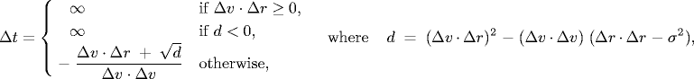
- Collision between particle and a wall. Given the position (rx, ry), velocity (vx, vy), and radius σ of a particle at time t, we wish to determine if and when it will collide with a vertical or horizontal wall.
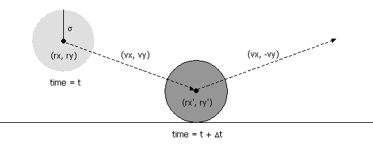
An analogous equation predicts the time of collision with a vertical wall.
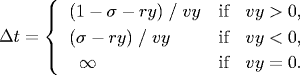
- Collision between two particles. Given the positions and velocities of two particles i and j at time t, we wish to determine if and when they will collide with each other.
σ2 = (rxi' - rxj' )2 + (ryi' - ryj' )2
During the time prior to the collision, the particles move in straight-line trajectories. Thus,
rxi' = rxi + Δt vxi, ryi' = ryi + Δt vyi
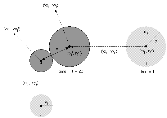
rxj' = rxj + Δt vxj, ryj' = ryj + Δt vyjSubstituting these four equations into the previous one, solving the resulting quadratic equation for Δt, selecting the physically relevant root, and simplifying, we obtain an expression for Δt in terms of the known positions, velocities, and radii.
If either Δv ⋅ Δr ≥ 0 or d < 0, then the quadratic equation has no solution for Δt > 0; otherwise we are guaranteed that Δt ≥ 0.
Collision resolution. In this section we present the physical formulas that specify the behavior of a particle after an elastic collision with a reflecting boundary or with another particle. For simplicity, we ignore multi-particle collisions. There are three equations governing the elastic collision between a pair of hard discs: (i) conservation of linear momentum, (ii) conservation of kinetic energy, and (iii) upon collision, the normal force acts perpendicular to the surface at the collision point. Physics-ly inclined students are encouraged to derive the equations from first principles; the rest of you may keep reading.
- Between particle and wall. If a particle with velocity (vx, vy) collides with a wall perpendicular to x-axis, then the new velocity is (-vx, vy); if it collides with a wall perpendicular to the y-axis, then the new velocity is (vx, -vy).
- Between two particles. When two hard discs collide, the normal force acts along the line connecting their centers (assuming no friction or spin). The impulse (Jx, Jy) due to the normal force in the x and y directions of a perfectly elastic collision at the moment of contact is:

and where mi and mj are the masses of particles i and j, and σ, Δx, Δy and Δ v ⋅ Δr are defined as above. Once we know the impulse, we can apply Newton's second law (in momentum form) to compute the velocities immediately after the collision.
vxi' = vxi + Jx / mi, vxj' = vxj - Jx / mj
vyi' = vyi + Jy / mi, vyj' = vyj - Jy / mj
Data format. Use the following data format. The first line contains the number of particles N. Each of the remaining N lines consists of 6 real numbers (position, velocity, mass, and radius) followed by three integers (red, green, and blue values of color). You may assume that all of the position coordinates are between 0 and 1, and the color values are between 0 and 255. Also, you may assume that none of the particles intersect each other or the walls.
N
rx ry vx vy mass radius r g b
rx ry vx vy mass radius r g b
rx ry vx vy mass radius r g b
rx ry vx vy mass radius r g b
Your task. Write a program MDSimulation.java that reads in a set of particles from standard input and animates their motion according to the laws of elastic collisions and event-driven simulation.
Perhaps everything below is just for the checklist??
Particle collision simulation in Java. There are a number of ways to design a particle collision simulation program using the physics formulas above. We will describe one such approach, but you are free to substitute your own ideas instead. Our approach involves the following data types: MinPQ, Particle, CollisionSystem, and Event.
- Priority queue. A standard priority queue where we can check if the priority queue is empty; insert an arbitrary element; and delete the minimum element.
- Particle data type. Create a data type to represent particles moving in the unit box. Include private instance variables for the position (in the x and y directions), velocity (in the x and y directions), mass, and radius. It should also have the following instance methods
- public Particle(...): constructor.
- public double collidesX(): return the duration of time until the invoking particle collides with a vertical wall, assuming it follows a straight-line trajectory. If the particle never collides with a vertical wall, return a negative number (or +infinity = DOUBLE_MAX or NaN???)
- public double collidesY(): return the duration of time until the invoking particle collides with a horizontal wall, assuming it follows a straight-line trajectory. If the particle never collides with a horizontal wall, return a negative number.
- public double collides(Particle b): return the duration of time until the invoking particle collides with particle b, assuming both follow straight-line trajectories. If the two particles never collide, return a negative value.
- public void bounceX(): update the invoking particle to simulate it bouncing off a vertical wall.
- public void bounceY(): update the invoking particle to simulate it bouncing off a horizontal wall.
- public void bounce(Particle b): update both particles to simulate them bouncing off each other.
- public int getCollisionCount(): return the total number of collisions involving this particle.
- Event data type. Create a data type to represent collision events. There are four different types of events: a collision with a vertical wall, a collision with a horizontal wall, a collision between two particles, and a redraw event. This would be a fine opportunity to experiment with OOP and polymorphism. We propose the following simpler (but somewhat less elegant approach).
- public Event(double t, Particle a, Particle b): Create a new event representing a collision between particles a and b at time t. If neither a nor b is null, then it represents a pairwise collision between a and b; if both a and b are null, it represents a redraw event; if only b is null, it represents a collision between a and a vertical wall; if only a is null, it represents a collision between b and a horizontal wall.
- public double getTime(): return the time associated with the event.
- public Particle getParticle1(): return the first particle, possibly null.
- public Particle getParticle2(): return the second particle, possibly null.
- public int compareTo(Object x): compare the time associated with this event and x. Return a positive number (greater), negative number (less), or zero (equal) accordingly.
- public boolean wasSuperveningEvent(): return true if the event has been invalidated since creation, and false if the event has been invalidated.
In order to implement wasSuperveningEvent, the event data type should store the collision counts of two particles at the time the event was created. The event corresponds to a physical collision if the current collision counts of the particles are the same as when the event was created.
- Particle collision system. The main program containing the event-driven simulation. Follow the event-driven simulation loop described above, but also consider collisions with the four walls and redraw events.
Data sets. Some possibilities that we'll supply.
- One particle in motion.
- Two particles in head on collision.
- Two particles, one at rest, colliding at an angle.
- Some good examples for testing and debugging.
- One red particle in motion, N blue particles at rest.
- N particles on a lattice with random initial directions (but same speed) so that the total kinetic energy is consistent with some fixed temperature T, and total linear momentum = 0. Have a different data set for different values of T.
- Diffusion I: assign N very tiny particles of the same size near the center of the container with random velocities.
- Diffusion II: N blue particles on left, N green particles on right assigned velocities so that they are thermalized (e.g., leave partition between them and save positions and velocities after a while). Watch them mix. Calculate average diffusion rate?
- N big particles so there isn't much room to move without hitting something.
- Einstein's explanation of Brownian motion: 1 big red particle in the center, N smaller blue particles.
Things you could compute.
- Brownian motion. In 1827, the botanist Robert Brown observed the motion of wildflower pollen grains immersed in water using a microscope. He observed that the pollen grains were in a random motion, following what would become known as Brownian motion. This phenomenon was discussed, but no convincing explanation was provided until Einstein provided a mathematical one in 1905. Einstein's explanation: the motion of the pollen grain particles was caused by millions of tiny molecules colliding with the larger particles. He gave detailed formulas describing the behavior of tiny particles suspended in a liquid at a given temperature. Einstein's explanation was intended to help justify the existence of atoms and molecules and could be used to estimate the size of the molecules. Einstein's theory of Brownian motion enables engineers to compute the diffusion constants of alloys by observing the motion of individual particles. Here's a flash demo of Einstein's explanation of Brownian motion from here.
- Free path and free time. Free path = distance a particle travels between collisions. Plot histogram. Mean free path = average free path length over all particles. As temperature increases, mean free path increases (holding pressure constant). Compute free time length = time elapsed before a particle collides with another particle or wall.
- Collision frequency. Number of collisions per second.
- Root mean-square velocity. Root mean-square velocity / mean free path = collision frequency. Root mean square velocity = sqrt(3RT/M) where molar gas constant R = 8.314 J / mol K, T = temperature (e.g., 298.15 K), M = molecular mass (e.g., 0.0319998 kg for oxygen).
- Maxwell-Boltzmann distribution. Distribution of velocity of particles in hard sphere model obey Maxwell-Boltzmann distribution (assuming system has thermalized and particles are sufficiently heavy that we can discount quantum-mechanical effects). Distribution shape depends on temperature. Velocity of each component has distribution proportional to exp(-mv_x^2 / 2kT). Magnitude of velocity in d dimensions has distribution proportional to v^(d-1) exp(-mv^2 / 2kT). Used in statistical mechanics because it is unwieldy to simulate on the order of 10^23 particles. Reason: velocity in x, y, and z directions are normal (if all particles have same mass and radius). In 2d, Rayleigh instead of Maxwell-Boltzmann.
- Pressure. Main thermodynamic property of interest = mean pressure. Pressure = force per unit area exerted against container by colliding molecules. In 2d, pressure = average force per unit length on the wall of the container.
- Temperature. Plot temperature over time (should be constant) = 1/N sum(mv^2) / (d k), where d = dimension = 2, k = Boltzmann's constant.
- Diffusion. Molecules travel very quickly (faster than a speeding jet) but diffuse slowly because they collide with other molecules, thereby changing their direction. Two vessels connected by a pipe containing two different types of particles. Measure fraction of particles of each type in each vessel as a function of time.
- Time reversibility. Change all velocities and run system backwards. Neglecting roundoff error, the system will return to its original state!
- Maxwell's demon. Maxwell's demon is a thought experiment conjured up by James Clerk Maxwell in 1871 to contradict the second law of thermodynamics. Vertical wall in middle with molecule size trap door, N particles on left half and N on right half, particle can only go through trap door if demon lets it through. Demon lets through faster than average particles from left to right, and slower than average particles from right to left. Can use redistribution of energy to run a heat engine by allowing heat to flow from left to right. (Doesn't violate law because demon must interact with the physical world to observe the molecules. Demon must store information about which side of the trap door the molecule is on. Demon eventually runs out of storage space and must begin erasing previous accumulated information to make room for new information. This erasing of information increases the entropy, requiring kT ln 2 units of work.)
Cell method. Useful optimization: divide region into rectangular cells. Ensure that particles can only collide with particles in one of 9 adjacent cells in any time quantum. Reduces number of binary collision events that must be calculated. Downside: must monitor particles as they move from cell to cell.
Extra credit. Handle multi-particle collisions. Such collisions are important when simulating the break in a game of billiards.
This assignment was developed by Ben Tsou and Kevin Wayne.Copyright © 2004.
Last modified on January 31, 2009.
Copyright © 2000–2019 Robert Sedgewick and Kevin Wayne. All rights reserved.
Monte Carlo Simulation
https://introcs.cs.princeton.edu/java/98simulation/
This section under major construction.
In 1953 Enrico Fermi, John Pasta, and Stanslaw Ulam created the first "computer experiment" to study a vibrarting atomic lattice. Nonlinear system couldn't be analyzed by classical mathematics.
Simulation = analytic method that imitates a physical system. Monte Carlo simulation = use randomly generated values for uncertain variables. Named after famous casino in Monaco. At essentially each step in the evolution of the calculation, Repeat several times to generate range of possible scenarios, and average results. Widely applicable brute force solution. Computationally intensive, so use when other techniques fail. Typically, accuracy is proportional to square root of number of repetitions. Such techniques are widely applied in various domains including: designing nuclear reactors, predicting the evolution of stars, forecasting the stock market, etc.
Generating random numbers. The math library function Math.random generate a pseudo-random number greater than or equal to 0.0 and less than 1.0. If you want to generate random integers or booleans, the best way is to use the library Random. Program RandomDemo.java illustrates how to use it.
Note that you should only create a new Random object once per program. You will not get more "random" results by creating more than one. For debugging, you may wish to produce the same sequence of pseudo-random number each time your program executes. To do this, invoke the constructor with a long argument.
The pseudo-random number generator will use 1234567 as the seed. Use SecureRandom for cryptographically secure pseudo-random numbers, e.g., for cryptography or slot machines.
Linear congruential random number generator. With integer types we must be cognizant of overflow. Consider a * b (mod m) as an example (either in context of a^b (mod m) or linear congruential random number generator: Given constants a, c, m, and a seed x[0], iterate: x = (a * x + c) mod m. Park and Miller suggest a = 16807, m = 2147483647, c = 0 for 32-bit signed integers. To avoid overflow, use Schrage's method.
Exercise: compute cycle length.
Library of probability functions. OR-Objects contains many classic probability distributions and random number generators, including Normal, F, Chi Square, Gamma, Binomial, Poisson. You can download the jar file here. Program ProbDemo.java illustrates how to use it. It generate one random value from the gamma distribution and 5 from the binomial distribution. Note that the method is called getRandomScaler and not getRandomScalar.
Queuing models. M/M/1, etc. A manufacturing facility has M identical machines. Each machine fails after a time that is exponentially distributed with mean 1 / μ. A single repair person is responsible for maintaining all the machines, and the time to fix a machine is exponentially distributed with mean 1 / λ. Simulate the fraction of time in which no machines are operational.
Diffusion-limited aggregation.
Diffuse = undergo random walk. The physical process diffusion-limited aggregation (DLA) models the formation of an aggregate on a surface, including lichen growth, the generation of polymers out of solutions, carbon deposits on the walls of a cylinder of a Diesel engine, path of electric discharge, and urban settlement.
The modeled aggregate forms when particles are released one at a time into a volume of space and, influenced by random thermal motion, they diffuse throughout the volume. There is a finite probability that the short-range attraction between particles will influence the motion. Two particles which come into contact with each other will stick together and form a larger unit. The probability of sticking increases as clusters of occupied sites form in the aggregate, stimulating further growth. Simulate this process in 2D using Monte Carlo methods: Create a 2D grid and introduce particles to the lattice through a launching zone one at a time. After a particle is launched, it wanders throughout with a random walk until it either sticks to the aggregate or wanders off the lattice into the kill zone. If a wandering particle enters an empty site next to an occupied site, then the particle's current location automatically becomes part of the aggregate. Otherwise, the random walk continues. Repeat this process until the aggregate contains some pre-determined number of particles. Reference: Wong, Samuel, Computational Methods in Physics and Engineering, 1992.
Program DLA.java simulates the growth of a DLA with the following properties. It uses the helper data type Picture.java. Set the initial aggregate to be the bottom row of the N-by-N lattice. Launch the particles from a random cell in top row. Assume that the particle goes up with probability 0.15, down with probability 0.35, and left or right with probability 1/4 each. Continue until the particles stick to a neighboring cell (above, below, left, right, or one of the four diagonals) or leaves the N-by-N lattice. The preferred downward direction is analogous to the effect of a temperature gradient on Brownian motion, or like how when a crystal is formed, the bottom of the aggregate is cooled more than the top; or like the influence of a gravitational force. For effect, we color the particles in the order they are released according to the rainbow from red to violet. Below are three simulations with N = 176; here is an image with N = 600.
 |
 |
 |
Brownian motion. Brownian motion is a random process used to model a wide variety of physical phenomenon including the dispersion of ink flowing in water, and the behavior of atomic particles predicted by quantum physics. (more applications). Fundamental random process in the universe. It is the limit of a discrete random walk and the stochastic analog of the Gaussian distribution. It is now widely used in computational finance, economics, queuing theory, engineering, robotics, medical imaging, biology, and flexible manufacturing systems. First studied by a Scottish botanist Robert Brown in 1828 and analyzed mathematically by Albert Einstein in 1905. Jean-Baptiste Perrin performed experiments to confirm Einstein's predictions and won a Nobel Prize for his work. An applet to illustrate physical process that may govern cause of Brownian motion.
Simulating a Brownian motion. Since Brownian motion is a continuous and stochastic process, we can only hope to plot one path on a finite interval, sampled at a finite number of points. We can interpolate linearly between these points (i.e., connect the dots). For simplicitly, we'll assume the interval is from 0 to 1 and the sample points t0, t1, ..., tN are equally spaced in this interval. To simulate a standard Brownian motion, repeatedly generate independent Gaussian random variables with mean 0 and standard deviation sqrt(1/N). The value of the Brownian motion at time i is the sum of the first i increments.
 |
 |
 |
Black-Scholes formula. Move to here?
Ising model. The motions of electrons around a nucleus produce a magnetic field associated with the atom. These atomic magnets act much like conventional magnets. Typically, the magnets point in random directions, and all of the forces cancel out leaving no overall magnetic field in a macroscopic clump of matter. However, in some materials (e.g., iron), the magnets can line up producing a measurable magnetic field. A major achievement of 19th century physics was to describe and understand the equations governing atomic magnets. The probability that state S occurs is given by the Boltzmann probability density function P(S) = e-E(S)/kT / Z, where Z is the normalizing constant (partition function) sum e-E(A)/kT over all states A, k is Boltzmann's constant, T is the absolute temperature (in degrees Kelvin), and E(S) is the energy of the system in state S.
Ising model proposed to describe magnetism in crystalline materials. Also models other naturally occurring phenomena including: freezing and evaporation of liquids, protein folding, and behavior of glassy substances.
Ising model. The Boltzmann probability function is an elegant model of magnetism. However, it is not practical to apply it for calculating the magnetic properties of a real iron magnet because any macroscopic chunk of iron contains an enormous number atoms and they interact in complicated ways. The Ising model is a simplified model for magnets that captures many of their important properties, including phase transitions at a critical temperature. (Above this temperature, no macroscopic magnetism, below it, systems exhibits magnetism. For example, iron loses its magnetization around 770 degrees Celsius. Remarkable thing is that transition is sudden.) reference
First introduced by Lenz and Ising in the 1920s. In the Ising model, the iron magnet is divided into an N-by-N grid of cells. (Vertex = atom in crystal, edge = bond between adjacent atoms.) Each cell contains an abstract entity known as spin. The spin si of cell i is in one of two states: pointing up (+1) or pointing down (-1). The interactions between cells is limited to nearest neighbors. The total magnetism of the system M = sum of si. The total energy of the system E = sum of - J si sj, where the sum is taken over all nearest neighbors i and j. The constant J measures the strength of the spin-spin interactions (in units of energy, say ergs). [The model can be extended to allow interaction with an external magnetic field, in which case we add the term -B sum of sk over all sites k.] If J > 0, the energy is minimized when the spins are aligned (both +1 or both -1) - this models ferromagnetism. if J < 0, the energy is minimized when the spins are oppositely aligned - this models antiferromagnetism.
Given this model, a classic problem in statistical mechanics is to compute the expected magenetism. A state is the specification of the spin for each of the N^2 lattice cells. The expected magnetism of the system E[M] = sum of M(S) P(S) over all states S, where M(S) is the magnetism of state S, and P(S) is the probability of state S occurring according to the Boltzmann probability function. Unfortunately, this equation is not amenable to a direct computational because the number of states S is 2N*N for an N-by-N lattice. Straightforward Monte Carlo integration won't work because random points will not contribute much to sum. Need selective sampling, ideally sample points proportional to e-E/kT. (In 1925, Ising solved the problem in one dimension - no phase transition. In a 1944 tour de force, Onsager solved the 2D Ising problem exactly. His solution showed that it has a phase transition. Not likely to be solved in 3D - see intractability section.)
Metropolis algorithm. Widespread usage of Monte Carlo methods began with Metropolis algorithm for calculation of rigid-sphere system. Published in 1953 after dinner conversation between Metropolis, Rosenbluth, Rosenbluth, Teller, and Teller. Widely used to study equilibrium properties of a system of atoms. Sample using Markov chain using Metropolis' rule: transition from A to B with probability 1 if Δ E <= 0, and with probability e-ΔE/kT if Δ E > 0. When applied to the Ising model, this Markov chain is ergodic (similar to Google PageRank requirement) so the theory underlying the Metropolis algorithm applies. Converges to stationary distribution.
Program Cell.java, State.java, and Metropolis.java implements the Metropolis algorithm for a 2D lattice. Ising.java is a procedural programming version. "Doing physics by tossing dice." Simulate complicated physical system by a sequence of simple random steps.
Measuring physical quantities. Measure magnetism, energy, specific heat when system has thermalized (the system has reached a thermal equilibrium with its surrounding environment at a common temperature T). Compute the average energy and the average magenetization over time. Also interesting to compute the variance of the energy or specific heat <c> = <E2> - <E>2, and the variance of the magnetization or susceptibility <Χ> = <M2> - <M>2. Determining when system has thermalized is a challenging problem - in practice, many scientists use ad hoc methods.
Phase transition. Phase transition occurs when temperature Tc is 2 / ln(1 + sqrt(2)) = 2.26918). Tc is known as the Curie temperature. Plot magnetization M (average of all spins) vs. temperature (kT = 1 to 4). Discontinuity of slope is signature of second order phase transition. Slope approaches infinity. Plot energy (average of all spin-spin interactions) vs. temperature (kT = 1 to 4). Smooth curve through phase transition. Compare against exact solution. Critical temperature for which algorithm dramatically slows down. Below are the 5000th sample trajectory for J/kT = 0.4 (hot / disorder) and 0.47 (cold / order). The system becomes magnetic as temperature decreases; moreover, as temperature decreases the probability that neighboring sites have the same spin increasing (more clumping).
Experiments.
- Start will above critical temperature. State converges to nearly uniform regardless of initial state (all up, all down, random) and fluctuates rapidly. Zero magnetization.
- Start well below critical temperature. Start all spins with equal value (all up or all down). A few small clusters of opposite spin form.
- Start well below critical temperature. Start with random spins. Large clusters of each spin form; eventually simulation makes up its mind. Equally likely to have large clusters in up or down spin.
- Start close to critical temperature. Large clusters form, but fluctuate very slowly.
 |
 |
Exact solution for Ising model known for 1D and 2D; NP-hard for 3d and nonplanar graphs.
Models phase changes in binary alloys and spin glasses. Also models neural networks, flocking birds, and beating heart cells. Over 10,000+ papers published using the Ising model.
Q + A
Exercises
- Print a random word. Read in a list of words (of unknown length) from standard input, and print out one of the N words uniformly at random. Do not store the word list. Instead, use Knuth's method: when reading in the ith word, select it with probability 1/i to be the new champion. Print out the word that survives after reading in all of the data.
- Random subset of a linked list. Given an array of N elements and an integer k ≤ N, construct a new array containing a random subset of k elements. Hint: traverse the array, either accepting each element with probability a/b, where a is the number of elements left to select, and b is the number of elements remaining.
Creative Exercises
- Random number generation. Can the following for computing a pseudo-random integer between 0 and N-1 fail? Math.random is guaranteed to return a floating point number greater than or equal to 0.0 and strictly less than 1.0.
double x = Math.random();
int r = (int) (x * N);
That is, can you find a real number x and an integer N for which r equals N?
Solution: No, it can't happen in IEEE floating point arithmetic. The roundoff error will not cause the result to be N, even if Math.random returns 0.9999999999.... However, this method does not produce integers uniformly at random because floating point numbers are not evenly distributed. Also, it involves casting and multiplying, which are excessive.
- Random number test. Write a program to plot the outcome of a boolean pseudo-random number generator. For simplicity, use (Math.random() < 0.5) and plot in a 128-by-128 grid like the following pseudorandom applet. Perhaps use LFSR or Random.nextLong() % 2.
- Sampling from a discrete probability distribution. Suppose that there are N events and event i occurs with probability pi, where p0 + p1 + ... + pN-1 = 1. Write a program Sample.java that prints out 1,000 sample events according to the probability distribution. Hint: choose a random number r between 0 and 1 and iterate from i = 0 to N-1 until p0 + p1 + ... + pi > r. (Be careful about floating point precision.)
- Sampling from a discrete probability distribution. Improve the algorithm from the previous problem so that it takes time proportional to log N to generate a new sample. Hint: binary search on the cumulative sums. Note: see this paper for a very clever alternative that generates random samples in a constant amount of time. Discrete.java is a Java version of Warren D. Smith's WDSsampler.c program.
- Sampling from a discrete probability distribution. Repeat the previous question but make it dynamic. That is, after each sample, the probabilities of some events might change, or there may be new events. Used in n-fold way algorithm, which is method of choice for kinetic Monte Carlo methods where one wants to simulate the kinetic evolution process. Typical application: simulating gas reacting with surface of a substrate where chemical reaction occur at different rates. Hint: use a binary search tree.
- Zipf distribution. Use the result of the previous exercise(s) to sample from the Zipfian distribution with parameter s and N. The distribution can take on integer values from 1 to N, and takes on value k with probability 1/k^s / sum_(i = 1 to N) 1/i^s. Example: words in Shakespeare's play Hamlet with s approximately equal to 1.
- Simulating a Markov chain. Write a program MarkovChain.java that simulates a Markov chain. Hint: you will need to sample from a discrete distribution.
- DLA with non-unity sticking probability Modify DLA.java so that the initial aggregate consists of several randomly spaced cells along the bottom of the lattice. This simulates string-like bacterial growth.
- DLA with non-unity sticking probability Modify DLA.java to allow a sticking probability less than one. That is, if a particle has a neighbor, then it sticks with probability p < 1.0; otherwise, it moves at random to a neighboring cell which is unoccupied. This results in a gives more clustered structure, simulating higher bond affinity between atoms.
- Symmetric DLA. Initialize the aggregate to be a single particle in the center of the lattice. Launch particles uniformly from a circle centered at the initial particle. Increase the size of the launch circle as the size of the aggregate increases. Name your program SymmetricDLA.java. This simulates the growth of an aggregate where the particles wander in randomly from infinity. Here are some tricks for speeding up the process.


- Variable sticking probability. A wandering particle which enters an empty site next to an occupied site is assigned a random number, indicating a potential direction in which the particle can move (up, down, left or right). If an occupied site exists on the new site indicated by the random number, then the particle sticks to the aggregate by occupying its current lattice site. If not, it moves to that site and the random walk continues. This simulates snowflake growth.
- Random walk solution of Laplace's equation. Numerically solve Laplace's equation to determine the electric potential given the positions of the charges on the boundary. Laplace's equation says that the gradient of the potential is the sum of the second partial derivatives with respect to x and y. See Gould and Tobochnik, 10.2. Your goal is to find the function V(x, y) that satisfies Laplace's equation at specified boundary conditions. Assume the charge-free region is a square and that the potential is 10 along the vertical boundaries and 5 along the horizontal ones. To solve Laplace's equation, divide the square up into an N-by-N grid of points. The potential V(x, y) of cell (x, y) is the average of the potentials at the four neighboring cells. To estimate V(x, y), simulate 1 million random walkers starting at cell (x, y) and continuing until they reach the boundary. An estimate of V(x, y) is the average potential at the 1 million boundary cells reached. Write a program Laplace.java that takes three command line parameters N, x, and y and estimates V(x, y) over an N-by-N grid of cells where the potential at column 0 and N is 10 and the potential at row 0 and N is 5.Remark: although the boundary value problem above can be solved analytically, numerical simulations like the one above are useful when the region has a more complicated shape or needs to be repeated for different boundary conditions.
simulated annealing
- Simulating a geometric random variable. If some event occurs with probability p, a geometric random variable with parameter p models the number N of independent trials needed between occurrence of the event. To generate a variable with the geometric distribution, use the following formula
N = ceil(ln U / ln (1 - p))
where U is a variable with the uniform distribution. Use the Math library methods Math.ceil, Math.log, and Math.random.
- Simulating an exponential random variable. The exponential distribution is widely used to model the the inter-arrival time between city buses, the time between failure of light bulbs, etc. The probability that an exponential random variable with parameter λ is less than x is F(x) = 1 - eλ x for x >= 0. To generate a random deviate from the distribution, use the inverse function method: output -ln(U) / λ where U is a uniform random number between 0 and 1.
- Poisson distribution. The Poisson distribution is useful in describing the fluctuations in the number of nuclei that decay in any particular small time interval.
public static int poisson(double c) { double t = 0.0; for (int x = 0; true; x++) { t = t - Math.log(Math.random()) / c; // sum exponential deviates if (t > 1.0) return x; } } - Simulating a Pareto random variable. The Pareto distribution is often used to model insurance claims damages, financial option holding times, and Internet traffic activity. The probability that a Pareto random variable with parameter a is less than x is F(x) = 1 - (1 + x)-a for x >= 0. To generate a random deviate from the distribution, use the inverse function method: output (1-U)-1/a - 1, where U is a uniform random number between 0 and 1.
- Simulating a Cauchy random variable. The density function of a Cauchy random variable is f(x) = 1/(Π(1 + x2)). The probability that a Cauchy random variable is less than x is F(x) = 1/Π (Π/2 + arctan(x)). To generate a random deviate from the distribution, use the inverse function method: output tan(Π(U - 1/2)), where U is a uniform random number between 0 and 1.
- Generate random point inside unit disc. Incorrect to choose set r uniformly between 0 and 1, θ uniformly between 0.0 and 2π, and use (x, y) = (r cosθ, r sinθ). If you do this, more points close to center of disc. Instead, set (x, y) = (√r cos&theta, √r sinθ) Alternatively, generate x and y uniformly between -1 and 1 and accept if x2 + y2 ≤ 1. Plot a random sequence of points using both methods and see the bias.
- Flipping bits. As part of a genetic algorithm, suppose you need to flip N bits independently, each with probability p, where p is some very small constant.
- Method 1: loop through N bits, generate a Bernouilli(p) random variable for each one and flip accordingly. Takes time proportional to N.
- Method 2: generate a Geometric(p) random variable X_0 and flip bit X_0; genereate another Geometric(p) random variable an flip bit X_0 + X_1, and so on. Takes time proportional to Np.
- Method 3: the number of bits to flip in Binomial(N, p). Determine how many bits to flip by approximating with a Gaussian(Np, sigma) random variable. Then flip Z bits, taking care not to avoid duplicates. Takes time proportional to Np, but less calls to transcendental functions.
- Random point inside N-dimensional sphere. Write a program InsideSphere.java that takes a command line parameter N and computes a random point inside an N-dimensional sphere with radius 1. Generate N uniform random variables deviates x1, ..., xN and use this point if
(x1)2 + ... + (xN)2 ≤ 1
Otherwise repeat.
- Random point on surface of an N-dimensional sphere. Write a program Sphere.java that takes a command line parameter N and computes a random point on the surface of an N-dimensional sphere with radius 1 using Brown's method. Brown's method is to compute N independent standard normal deviates x1, xN. Then
( x1/r, x2/r, ..., xN/r ), where r = sqrt((x1)2 + ... + (xN)2)
has the desired distribution. Use Exercise xyz from Section 3 to compute standard normal deviates.
- Potts model. The Potts model is a variant of the Ising model where each site has q possible directions. (q = 2 corresponds to Ising) The total energy of the system E = sum of - J sigma(si, sj) over all neighbors. The Kronecker delta function δ(x, y) = 1 if x = y and 0 otherwise.
- 2D Brownian motion. Simulate diffusion of particles in a fluid. Write a data type BrownianParticle.java that represents a particle undergoing a Brownian motion in two dimensions. To do this, simulate two indepedent Brownian motions X(t) and Y(t), and plot (X(t), Y(t)). Create a client program that takes a command line integer N, creates N particles at the origin, and simulates a Brownian motion for the N particles.
- Brownian bridge. A Browian bridge is a constratined Brownian motion, which is required to begin at the origin at time 0, and end at the origin at time T. If X(t) is a Brownian motion then Z(t) = X(t) - (t/T)X(T) is such a process. To plot, store the intermediate values X(t) and plot after you've computed X(T).
- Rainbow. In 1637 Rene Descartes discovered the first scientific explanation for the formation of rainbows. His method involved tracing the internal reflections when a light ray is sent through a a spherical raindrop. Simulate the generation of a rainbow according to model of large number of parallel rays hitting a spherical raindrop. When a light ray hit a raindrop, the ray is reflected and refracted. We use the HSB color format, and choose the hue h at random between 0 (red) and 1 (violet). We use 1.33 + 0.06 * h for the refraction index of hue h. For each ray, we plot a single point of light, according to physical laws of refraction and reflection. Each point of light is then plotted in a random color that the observer will see, either in the primary or secondary rainbow. To perform the simulation, we choose one of the 7 colors uniformly at random. Then, we choose a point (x, y) in the unit circle, centered at (0, 0) and set the impact parameter r = sqrt(x2 + y2). The angle of incidence θi = arcsin(r) and, by Snell's law, the angle of refraction θr = arcsin (r / n), where n is the refraction index. If the light ray is totally reflected only once, it emerges at an angle of θp = 4θr - 2θi, contributing to the primary rainbow. If the light ray is totally reflected a second time, it emerges at an angle of θp = 6θr - 2θi - π, contributing to the secondary rainbow. The intensities Ip and Is of the primary and secondary rays are calculated according to the following transmission and reflection formulas for electromagnetic waves across the boundary of two media.
Ip = 1/2 (s(1-s)2 + p(1-p)2)
Is = 1/2 (s2(1-s)2 + p2(1-p)2)
p = (sin(θi-θr)/sin(θi+θr))2
r = (tan(θi-θr)/tan(θi+θr))2
The color intensities Ip and Is are used to determine the saturation in the HSB color format. Program Rainbow.java simulates this process.

Last modified on January 31, 2009.
Copyright © 2000–2019 Robert Sedgewick and Kevin Wayne. All rights reserved.
Is a New Particle Changing the Fate of the Universe?
https://www.space.com/new-particle-changing-fate-of-universe.html?utm_source=notification
Astronomers around the world are in a bit of a tizzy because they can't seem to agree about how fast the universe is expanding.
Ever since our universe emerged from an explosion of a tiny speck of infinite density and gravity, it has been ballooning, and not at a steady rate, either — the expansion of the universe keeps getting faster.
But how quickly it's expanding has been up for a dizzying debate. Measurements of this expansion rate from nearby sources seem to be in conflict with the same measurement taken from distant sources. One possible explanation is that, basically, something funky is going on in the universe, changing the expansion rate.
And one theorist has proposed that a brand-new particle has emerged and is altering the future destiny of our entire cosmos.
Related: How the Universe Stopped Making Sense
Hubble, Hubble, toil and trouble
Astronomers have devised multiple clever ways of measuring what they call the Hubble parameter, or Hubble constant (denoted for the folks with busy lives as H0). This number represents the expansion rate of the universe today.
One way to measure the expansion rate today is to look at nearby supernovas, the explosion of gas and dust launched from the universe's largest stars upon their death. There's a particular kind of supernova that has a very specific brightness, so we can compare how bright they look to how bright we know they're supposed to be and calculate the distance. Then, by looking at the light from the supernova's host galaxy, astrophysicists can also calculate how fast they are moving away from us. By putting all the pieces together, we then can calculate the universe's expansion rate.
But there's more to the universe than exploding stars. There's also something called the cosmic microwave background, which is the leftover light from just after the Big Bang, when our universe was a mere baby, only 380,000 years old. With missions like the Planck satellite tasked with mapping this remnant radiation, scientists have incredibly precise maps of this background, which can be used to get a very accurate picture of the contents of the universe. And from there, we can take those ingredients and run the clock forward with computer models and be able to say what the expansion rate should be today — assuming that the fundamental ingredients of the universe haven’t changed since then.
Related: From Big Bang to Present: Snapshots of Our Universe Through Time
These two estimates disagree by enough to make people a little bit worried that we're missing something.
Look to the dark side
Perhaps, one or both measurements are incorrect or incomplete; plenty of scientists on either side of the debate are slinging the appropriate amount of mud at their opponents. But if we assume that both measurements are accurate, then we need something else to explain the different measurements. Since one measurement comes from the very early universe, and another comes from more relatively recent time, the thinking is that maybe some new ingredient in the cosmos is altering the expansion rate of the universe in a way that we didn’t already capture in our models.
And what's dominating the expansion of the universe today is a mysterious phenomenon that we call dark energy. It's an awesome name for something we basically don't understand. All we know is that the expansion rate of the universe today is accelerating, and we call the force driving this acceleration "dark energy."
In our comparisons from the young universe to the present-day universe, physicists assume that dark energy (whatever it is) is constant. But with this assumption, we have the present disagreement, so maybe dark energy is changing.
I guess it's worth a shot. Let’s assume that dark energy is changing.
Scientists have a sneaking suspicion that dark energy has something to do with the energy that's locked into the vacuum of space-time itself. This energy comes from all of the “quantum fields” that permeate the universe.
In modern quantum physics, every single kind of particle is tied to its own particular field. These fields wash through all of space-time, and sometimes bits of the fields get really excited in places, becoming the particles that we know and love — like electrons and quarks and neutrinos. So all the electrons belong to the electron field, all the neutrinos belong to the neutrino field, and so on. The interaction of these fields form the fundamental basis for our understanding of the quantum world.
And no matter where you go in the universe, you can’t escape the quantum fields. Even when they’re not vibrating enough in a particular location to make a particle, they’re still there, wiggling and vibrating and doing their normal quantum thing. So these quantum fields have a fundamental amount of energy associated with them, even in the bare empty vacuum itself.
Related: The 11 Biggest Unanswered Questions About Dark Matter
If we want to use the exotic quantum energy of the vacuum of space-time to explain dark energy, we immediately run into problems. When we perform some very simple, very naive calculations of how much energy there is in the vacuum due to all the quantum fields, we end up with a number that is about 120 orders of magnitude stronger than what we observe dark energy to be. Whoops.
On the other hand, when we try some more sophisticated calculations, we end up with a number that is zero. Which also disagrees with the measured amount of dark energy. Whoops again.
So no matter what, we have a really hard time trying to understand dark energy through the language of the vacuum energy of space-time (the energy created by those quantum fields). But if these measurements of the expansion rate are accurate and dark energy really is changing, then this might give us a clue into the nature of those quantum fields. Specifically, if dark energy is changing, that means that the quantum fields themselves have changed.
A new enemy appears
Advertisement
In a recent paper published online in the preprint journal arXiv, theoretical physicist Massimo Cerdonio at the University of Padova has calculated the amount of change in the quantum fields needed to account for the change in dark energy.
If there is a new quantum field that's responsible for the change in dark energy, that means there is a new particle out there in the universe.
And the amount of change in dark energy that Cerdonio calculated requires a certain kind of particle mass, which turns out to be roughly the same mass of a new kind of particle that's already been predicted: the so-called axion. Physicists invented this theoretical particle to solve some problems with our quantum understanding of the strong nuclear force.
This particle presumably appeared in the very early universe, but has been "lurking" in the background while other forces and particles controlled the direction of the universe. And now it's the axion's turn ...
Even so, we've never detected an axion, but if these calculations are correct, then that means that the axion is out there, filling up the universe and its quantum field. Also, this hypothetical axion is already making itself noticeable by changing the amount of dark energy in the cosmos. So it could be that even though we've never seen this particle in the laboratory, it's already altering our universe at the very largest of scales.
- 11 Fascinating Facts About Our Milky Way Galaxy
- Big Bang to Civilization: 10 Amazing Origin Events
- Spaced Out! 101 Astronomy Photos That Will Blow Your Mind
Originally published on Live Science.
Need more space? Subscribe to our sister title "All About Space" Magazine for the latest amazing news from the final frontier!
(Image credit: All About Space)
Have a news tip, correction or comment? Let us know at
https://videos.space.com/m/X9nG9n6P/hubbles-contentious-constant?list=9wzCTV4g
Planet Earth: Life: S1 Ep8 - Creatures of the Deep

Planet Earth: Creatures of the deep


Blue Whales
https://www.worldwildlife.org/species/blue-whale

The blue whale is the largest animal on the planet, weighing as much as 200 tons (approximately 33 elephants). The blue whale has a heart the size of a Volkswagen Beetle. Its stomach can hold one ton of krill and it needs to eat about four tons of krill each day. They are the loudest animals on Earth and are even louder than a jet engine. Their calls reach 188 decibels, while a jet reaches 140 decibels. Their low frequency whistle can be heard for hundreds of miles and is probably used to attract other blue whales.
https://en.wikipedia.org/wiki/Blue_whale
Blue whales were abundant in nearly all the oceans on Earth until the beginning of the twentieth century. For over a century, they were hunted almost to extinction by whaling until protected by the international community in 1966. A 2002 report estimated there were 5,000 to 12,000 blue whales worldwide,[3] in at least five populations. The IUCN estimates that there are probably between 10,000 and 25,000 blue whales worldwide today.[1] Before whaling, the largest population was in the Antarctic, numbering approximately 239,000 (range 202,000 to 311,000).[8] There remain only much smaller (around 2,000) concentrations in each of the eastern North Pacific, Antarctic, and Indian Ocean populations. There are two more groups in the North Atlantic, and at least two in the Southern Hemisphere. The Eastern North Pacific blue whale population had rebounded by 2014 to nearly its pre-hunting population.[9]
PROTECTING WILDLIFE FOR A HEALTHY PLANET

Planet Earth: Life: Fish


Clownfish Talk Their Way Out of Conflict

Solve quad eq
https://www.tiger-algebra.com/drill/3x2_11x_4=0/
3x2+11x+4=0
Two solutions were found :
- x =(-11-√73)/6=-3.257
- x =(-11+√73)/6=-0.409
Reformatting the input :
Changes made to your input should not affect the solution:
(1): "x2" was replaced by "x^2".
Step by step solution :
Step 1 :
Equation at the end of step 1 :
(3x2 + 11x) + 4 = 0
Step 2 :
Trying to factor by splitting the middle term
The first term is, 3x2 its coefficient is 3 .
The middle term is, +11x its coefficient is 11 .
The last term, "the constant", is +4
Step-1 : Multiply the coefficient of the first term by the constant 3 • 4 = 12
Step-2 : Find two factors of 12 whose sum equals the coefficient of the middle term, which is 11 .
| -12 | + | -1 | = | -13 | ||
| -6 | + | -2 | = | -8 | ||
| -4 | + | -3 | = | -7 | ||
| -3 | + | -4 | = | -7 | ||
| -2 | + | -6 | = | -8 | ||
| -1 | + | -12 | = | -13 | ||
| 1 | + | 12 | = | 13 | ||
| 2 | + | 6 | = | 8 | ||
| 3 | + | 4 | = | 7 | ||
| 4 | + | 3 | = | 7 | ||
| 6 | + | 2 | = | 8 | ||
| 12 | + | 1 | = | 13 |
Observation : No two such factors can be found !!
Conclusion : Trinomial can not be factored
Equation at the end of step 2 :
3x2 + 11x + 4 = 0
Step 3 :
Parabola, Finding the Vertex :
3.1 Find the Vertex of y = 3x2+11x+4
Parabolas have a highest or a lowest point called the Vertex . Our parabola opens up and accordingly has a lowest point (AKA absolute minimum) . We know this even before plotting "y" because the coefficient of the first term, 3 , is positive (greater than zero).
Each parabola has a vertical line of symmetry that passes through its vertex. Because of this symmetry, the line of symmetry would, for example, pass through the midpoint of the two x -intercepts (roots or solutions) of the parabola. That is, if the parabola has indeed two real solutions.
Parabolas can model many real life situations, such as the height above ground, of an object thrown upward, after some period of time. The vertex of the parabola can provide us with information, such as the maximum height that object, thrown upwards, can reach. For this reason we want to be able to find the coordinates of the vertex.
For any parabola,Ax2+Bx+C,the x -coordinate of the vertex is given by -B/(2A) . In our case the x coordinate is -1.8333
Plugging into the parabola formula -1.8333 for x we can calculate the y -coordinate :
y = 3.0 * -1.83 * -1.83 + 11.0 * -1.83 + 4.0
or y = -6.083
Parabola, Graphing Vertex and X-Intercepts :
Root plot for : y = 3x2+11x+4
Axis of Symmetry (dashed) {x}={-1.83}
Vertex at {x,y} = {-1.83,-6.08}
x -Intercepts (Roots) :
Root 1 at {x,y} = {-3.26, 0.00}
Root 2 at {x,y} = {-0.41, 0.00} Solve Quadratic Equation by Completing The Square
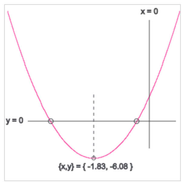
3.2 Solving 3x2+11x+4 = 0 by Completing The Square .
Divide both sides of the equation by 3 to have 1 as the coefficient of the first term :
x2+(11/3)x+(4/3) = 0
Subtract 4/3 from both side of the equation :
x2+(11/3)x = -4/3
Now the clever bit: Take the coefficient of x , which is 11/3 , divide by two, giving 11/6 , and finally square it giving 121/36
Add 121/36 to both sides of the equation :
On the right hand side we have :
-4/3 + 121/36 The common denominator of the two fractions is 36 Adding (-48/36)+(121/36) gives 73/36
So adding to both sides we finally get :
x2+(11/3)x+(121/36) = 73/36
Adding 121/36 has completed the left hand side into a perfect square :
x2+(11/3)x+(121/36) =
(x+(11/6)) • (x+(11/6)) =
(x+(11/6))2
Things which are equal to the same thing are also equal to one another. Since
x2+(11/3)x+(121/36) = 73/36 and
x2+(11/3)x+(121/36) = (x+(11/6))2
then, according to the law of transitivity,
(x+(11/6))2 = 73/36
We'll refer to this Equation as Eq. #3.2.1
The Square Root Principle says that When two things are equal, their square roots are equal.
Note that the square root of
(x+(11/6))2 is
(x+(11/6))2/2 =
(x+(11/6))1 =
x+(11/6)
Now, applying the Square Root Principle to Eq. #3.2.1 we get:
x+(11/6) = √ 73/36
Subtract 11/6 from both sides to obtain:
x = -11/6 + √ 73/36
Since a square root has two values, one positive and the other negative
x2 + (11/3)x + (4/3) = 0
has two solutions:
x = -11/6 + √ 73/36
or
x = -11/6 - √ 73/36
Note that √ 73/36 can be written as
√ 73 / √ 36 which is √ 73 / 6
Solve Quadratic Equation using the Quadratic Formula
3.3 Solving 3x2+11x+4 = 0 by the Quadratic Formula .
According to the Quadratic Formula, x , the solution for Ax2+Bx+C = 0 , where A, B and C are numbers, often called coefficients, is given by :
- B ± √ B2-4AC
x = ————————
2A
In our case, A = 3
B = 11
C = 4
Accordingly, B2 - 4AC =
121 - 48 =
73
Applying the quadratic formula :
-11 ± √ 73
x = ——————
6
√ 73 , rounded to 4 decimal digits, is 8.5440
So now we are looking at:
x = ( -11 ± 8.544 ) / 6
Two real solutions:
x =(-11+√73)/6=-0.409
or:
x =(-11-√73)/6=-3.257
Two solutions were found :
- x =(-11-√73)/6=-3.257
- x =(-11+√73)/6=-0.409
Computing with SciPy


Transform Science - Enthought


MONTE Python for Deep Space Navigation | SciPy 2016 | Jonathon Smith
Restored Apollo 11 Moonwalk - Original NASA EVA Mission Video - Walking on the Moon
Crash Course on Our Solar System & Beyond
How Earth Moves
Scott Manley - Orbital Dynamics
Jon Toellner - Orbital Dynamics
Orbital Dynamics - Parts 1 through 19 but missing parts
\\\
\\\\
\\\
What hypnosis does to your brain, and how it can improve your health Read more:
The history of hypnotherapy is riddled with hucksters, but it can provide real benefits – from weight loss to managing pain. Why modern medicine is starting to take it seriously
“HONESTLY, I wondered whether I was actually in labour, because surely it was meant to be more painful than this.” That’s Shona, describing the recent birth of her daughter. Her secret? Hypnosis. During pregnancy, she learned how to hypnotise herself into a state of mind that allowed her to minimise the pain of labour and, in her own words, “quite enjoy the whole thing”.
The word hypnosis may call to mind a swinging watch or an entertainer getting people to believe they are naked on stage for an audience’s amusement. Its history is one of sorcery and magic, tales of the occult and exploitative charlatans. Practitioners are rarely doctors or counsellors, clinical trials struggle to get funded and there is still no regulatory authority that monitors the practice.
Yet despite these issues, people are turning to the technique to help with everything from labour to hot flushes, anxiety and chronic pain, and a growing body of research is starting to confirm its benefits. We are also beginning to get a handle on how it actually works and what happens in the brain during hypnosis.
The result is that how we define hypnosis is changing, and its use in mainstream medicine is increasing. The UK’s Royal College of Midwives now accredits hypnobirthing courses and funds training in the technique. Some anaesthetists now include hypnosis in their toolkit, and it is even being touted as a solution for the opioid addiction crisis. Hypnosis is certainly no cure-all, but learning what works, why it works and how to do it ourselves may …

Go Beyond Technica

What is Technica?
Technica is the world’s largest all-women and nonbinary hackathon, hosted annually at the University of Maryland.
Over the duration of 24 hours, women and non-binary people are immersed in tech culture and encouraged to exercise their imagination to create interesting and innovative hacks.
This year’s theme is “Go Beyond”. At Technica, we want to see women and non-binary folks thrive and go beyond society’s expectations for them. We encourage all attendees to take your tech journey beyond Technica. Don’t stop at our hackathon, attend others and keep creating. Technica is meant to catapult you further in your career, and help you to continue achieving. As you advance in your career, go beyond your duties at work, become a mentor and help to advance the next generation of women in tech. Whatever your goals and aspirations, remember you can always #GoBeyond.
Empowering our Community to Make the New Normal
https://techtogether.io/
Our Chapters Host Hackathons
Across the Country
TechTogether is using the power of community and research to build a gender-diverse future in technology.
NEWSROOM
Boston Globe
Beyond the Straight and Narrow: Tech Sector Pushed to Accommodate Those Who Reject Strict Gender Norms
BostInno
BostInno’s 2018 50 On Fire
Untold Business
TechTogether: Blazing a Trail for Women in Technology & Female-Centric Hackathons
CBC
SheHacks: A 36-Hour Hackathon for Women
Boston Herald
Women feel welcome to code at SheHacks
Don't miss out when
hackathon applications go live!
Subscribe to be the first know about exclusive TechTogether events, jobs opportunities, and contests. This is not a monthly newsletter that will clog your inbox.

Seeing 2019: The Visual Trend Forecast from Adobe Stock

As designers and brands know, we live in a fast-paced, intensely visual age, which means that images are one of the most important ways brands connect with consumers. That’s the reason visual fluency — the ability to see visual trends coming and understand what they mean to consumers — is so important. And it’s the purpose behind Adobe Stock’s Visual Trends. Our trend reports help the creative community spot trends as they’re evolving, understand what they mean to consumers, and build on them for maximum impact.
In 2019, our visual landscape will reflect far more than fleeting fads, likes, and shares. We’ll be surrounded by images that capture passionate, beautiful, contentious, messy cultural conversations about values, how we express our individuality and experiences, and how we find refuge in tumultuous times.
The Adobe Stock team looked around the world, from fashion runways and art galleries to the business world, pop culture, and social media — all with the goal of uncovering the major visual trends that will shape the year.
Here’s an early peek at the trends we’re forecasting for 2019:
Natural Instincts

As technology increases in our lives and more of our days are spent in the digital realm, we’re feeling increasingly distant from the physical world. This steady shift is leading more people to consciously (or subconsciously) seek balance through nature. Artists like Adobe Stock Premium contributor Archan Nair are part of a movement of creatives taking inspiration from the mysteries of the natural world. Archan’s illustrations bring together surrealism, mysticism, and organic forms to explore the interconnectedness between humans and the planet.
This desire to connect with nature is shaping consumer behavior, too. For example, according to NPD Group, nearly half of U.S. consumers now actively seek natural ingredients in the products they choose. Beyond contents, consumers are also tuned into how ingredients are sourced and how brands communicate. The Global Wellness Institute reports that the fastest-growing portion of the $999 billion wellness and beauty industry is “clean beauty” — products that are ethical, sustainable, and transparent. Major retailers from Nordstrom and Barney’s to Sephora are responding, giving more of their space over to natural brands.

Along with this desire for a natural refuge, consumers are also looking for brands to satisfy their spiritual needs. Retailers are responding with spaces that include natural elements for a serene shopping aesthetic. Spiritual wellness events, such as LA’s monthly Conscious Family Dinners, are selling out. And companies like Moon Bath and Zephorium blur the lines between beauty, healing, and spirituality, offering products that promise all of the above.
In the visual world, designers are focusing on aspirational images with natural elements and celebrations of physical, emotional, and spiritual wellness.
Creative Democracy

We’re no longer waiting for creatives to shape our visual worlds — instead, people are using technology to elevate and share their own unpolished, raw, authentic moments in full, vivid color. Each day, 95 million photos are uploaded to Instagram, and people watch 100 million hours of video content on Facebook. Gen Z and Millennials are leading the charge but all ages are in on it, powered by mobile-first platforms that allow on-the-go content and livestreams on social media.
Brands are finding clever ways to harness our desire to create our own images. For example, clothing company American Eagle launched its #aeriereal campaign, asking women to post unretouched photos of themselves and celebrate body positivity. And furniture companies from West Elm to Wayfair invite users to post photos of their new products, letting consumers see how they look in a real home.

Tools and communities are emerging to embrace this new creative impulse too, like our partners at GoPro, and Adobe’s own Project Rush, which gives creatives of all generations the opportunity to create, edit, and share videos, across devices.
Diversity rules in creative democracy — both in front of the lens and behind it. Visually, creative democracy is all about unstudied images, bright colors, diverse subjects, and video that moves people.
Disruptive Expression

People are ready to have their voices heard. Whether it’s in creative play or fierce political resistance, images of extreme self-expression resonate. Our social feeds are full of marching protesters and impromptu political speeches. Brands are tapping into the energy, borrowing the visual language of protest for shop windows and clothing lines. And the moment feels so significant that galleries, from the Museum of the City of New York to the Smithsonian’s National Museum of American History, are collecting protest signs for future exhibits.

Even when there’s no political agenda, the new self-expression is all about inclusive, unapologetic, eye-catching visuals that cut through the noise. The images range from haunting and hypnotizing, like luxury fashion house Balenciaga’s jaw-droppingly bendable models, to shiny and playful, like the boom of Instagram posts bedazzled with the KiraKira app.
In the visual context, disruptive expression means embracing a wide range of identities, celebrating fearless individuality, and forgoing the light touch in favor of power and intensity.
Brand Stand

Consumers, especially Gen Z and millennials, want more from brands than just products — they’re giving their loyalty to companies with stated values and a commitment to transparency. A recent study found that nearly half of millennials think CEOs themselves ought to take a stand on social issues.
Some brands are taking headline-grabbing action to show their values. Consider Patagonia’s lawsuit against the president, which seeks to protect national monuments, or the companies that joined a legal fight against North Carolina’s bathroom bill.

Other brands are helping consumers become more ethically aware themselves. The innovative financial firm Aspiration, for example, created a program to help consumers match their day-to-day spending to their ethical beliefs.
To keep up with this trend, brands will need to communicate a meaningful, coherent social purpose around big issues, such as social justice and conservation. In the visual realm, this means that stunning, powerful representations of causes and popular issues on a global scale will have a big impact on viewers.
In fact, for some, the activism is in the imagery itself. The Ocean Agency’s collection on Adobe Stock, for example, invites viewers to experience the rarely seen beauty in the underwater world. “Ninety-nine percent of people don’t dive — and probably never will,” shares the company’s founder, Richard Vevers. “That’s why imagery is so important when it comes to ocean conservation. Our job is to take imagery that excites the world, to engage people with the most magical part of our planet — our underwater world — and through imagery get them supporting the fight to save it.”
Throughout the year, we’ll zoom in on each of these emerging trends, tracing their roots, exploring how they touch our everyday lives, and giving designers and brands the context they need to make the trends their own. We’ll also talk with Adobe Stock artists whose work embraces the trends and pushes their creative edges.
Stay with us all year as we dig deeper.
Karen Salmansohn
Karen Salmansohn
multi best selling author
award winning designer
Oprah columnist
over 1.5 million fans


#1 NEW RELEASE! Relax. Focus. Sleep.
Get ready to feel relaxed and happy. "Instant Calm" will give you simple & fun 2-minute meditations to help you stay calm and focused – even in tough times. LEARN MORE!
Live a life you love!
Enjoy Karen’s top shared articles and original quote posters!
Remember Golden Girls - and how those older friends cohoused in a community together? Well, senior cohousing with friends is[...]
After the death of a loved one, do you ever feel like they are communicating to you through strange signs[...]
If you're dealing with a challenge and feel stuck in a negative thought loop, I have a helpful tool. Read[...]
I believe you don't meet people by accident. People come into your life for a reason. Yes, even the crummy[...]
Improve your life in under 10 minutes a day!
Teach your old brain new tricks

Meet Karen Salmansohn! She has close to 2 million online fans and a celebrity following. She’s the founder of NotSalmon and NotSalmon Courses – plus, a multi best selling author with close to 2 million books sold nationally and internationally – a columnist for Oprah and Psychology Today – and an award winning designer of books, posters, jewelry and videos.
Her mission: To offer you easy-to-understand insights and tools to empower you to bloom into your happiest, highest potential self. She uses playful analogies, feisty humor, and stylish graphics to distill big ideas.
Snag these freebies!
Get simple research-based tools to create a life you love!

Happiness
Learn how to think, act and react in new ways to old issues – and start feeling a heck of a lot happier!

Health
You can age quickly or slowly. It’s your choice. Learn research based longevity tools in this bestselling book.

Love
Grab my Oprah-recommended tools and learn to date and mate in far happier and longer-lasting ways.

Success
It’s not what you got, it’s how you package it! Create a stand-out brand! Turn your passions into profits!
As seen in...
Reader Favorites
Are narcissists happy? Do wrong doers and bullies feel happiness - after wreaking unhappiness wherever they go? Do narcissists suffer?[...]
When your heart is broken, you can feel like your whole life is broken. These 4 tools will help you[...]
Do you keep attracting the wrong partners? Do you feel like you are wearing a kick me sign on your[...]
Do you tend to say I think or I feel? There's a big difference between thinking and feeling. Find out[...]
Want to know how to deal with an enemy or toxic person so they don't get to you? This is[...]
Kids hate it when mom and dad nag. Parents don't want to be nagging their children either. Here's a parenting[...]
Most people miss this important red flag in love - because it originally shows up as something you think you[...]
Check out this interesting emotional eating research. You'll learn an unusual way for how to best stop emotional eating -[...]
Join over 1.5 million loyal fans!
My research-backed happiness tools have been featured on CNN, Oprah, Psychology Today, The Today Show, etc – and will empower you to live a life of love!
No SPAM, ever! Read the Privacy Policy for more information.

NAN NEWARK TECH WORLD
Mission
Living in an increasingly digital world means broader access to almost all of life’s needs. Everything from shopping, banking, paying bills, studying, and applying for a job can all be done electronically. While the ease of access seems like a good enough reason to buy into computer Internet and Broadband technology, we know there are still many in minority and low-income communities who have not become adopters of technology and all that it has to offer. The resistance to use the Internet and computers in any form to solve many of life’s problems or create an easier lifestyle also creates barriers for the vast entrepreneurial opportunities that exist in the technology industry. The future of jobs lies heavily in this field and with a projected shortage of prepared workers, we know that many of the people who are not yet using broadband or using it in a limited capacity will be left out of the many opportunities that will exist.
National Action Network sees a chance to engage local leaders and communities to close the digital divide and bring access and opportunity to communities who are being left behind.
Goal
NAN 2016 Technology Tour Expands To Newark, New Jersey
Newark based Tech World features three (4) 21st century classroom learning environments outfitted with state-of-the-arts computer workstations in each classroom. Tech World is strategically located to have its broadest impact on Newark citizens with an administrative staff to address the training needs of Newark Citizens. The program dovetails with the White House’s Computer Science for all initiative where Newark students between the ages of 8-14 will become one of the primary beneficiaries of Tech World’s after-school computer science training program.
Newark youth will be offered programs in STEM, STEAM, Robotic, coding and software development (working with the Newark’s rich college community) while young adults and seniors will be able to pursue and engage in basic and intermediate computer training skills and other technology programs.
By hosting digital literacy sessions, hackathons, technology career events, and connecting students and adults with tech innovators in their communities, Tech World is bridging the divide through information. By partnering with local businesses and/or other partners like churches, Tech World also seeks ways to donate new technology to people within the community who are active in the Tech World programs. Through the education, connection to technology professionals and access to equipment, we address the technology divide in Newark.

hackathons
Talking About Diversity Again…At Hackathons?
May 31, 2018 · 6 min read
We were once asked by a competitor, why do we have diversity initiatives for the hackathon when it is ‘irrelevant’?
I understand the frustration from this competitor — the idea of giving somebody else an unfair advantage, or maybe the idea of taking away opportunities [from others] for the sake of quotas?
Considering the way technology is integrated throughout our daily lives, how it will define our future, and the growth of this industry, I find it very difficult to call these initiatives ‘irrelevant’. The lack of diverse representation in technology has very real and serious impacts on not only the industry itself but also the products that our society consumes as well.
Diversity in IT is a multi-faceted problem, and you can see this in:
- The blame we are placing on the underrepresented groups for their lack of representation (see: when marketing stopped women coding, alarmingly low numbers of Black/Latino/Indigenous people in the North American Tech Industry, college affordability becoming increasingly difficult for low-income or first-generation students).
- Areas where the product shows a bias of homogenous teams who created it (like the time when facial recognition thought a Chinese man’s eyes were closed, or when face-tracking software was unable to recognise black people because it was trained with white engineers).
- The drop out rates of people who fall in these groups because of divisive, toxic work cultures, and bullying in the workforce.
Not to mention there’s also the way we bring up our children (and before you tell me something like women just ‘aren’t interested’ or are ‘biologically incapable’, please see the: 70% of STEM grads in Iran who are women and the 45% of CS degree holders in India who are women).
We need more role models, and to emphasise the benefits, like increased creativity, productivity, and efficiency of teams.
Perhaps you might ask, well on a more granular level, where we’re talking about tertiary level students who are already in the pipeline, likely to get a job in technology, and have ‘no barrier’ to entry (because they are already ‘in’), why would an event care about diversity statistics?
Here’s some food for thought:
- Hackathons are intimidating. Regardless of your background, the idea of attending a competition (especially with strangers) requires a lot of courage. It is very understandable that for a lot of people, the uncomfortable idea of attending alone is more than enough to get rid of the idea of attending altogether.
- This is even more prevalent for underrepresented students who perceive their skills to be lower than it actually is.
- For a lot of students, what they see at extra-curricular events is what they expect in the industry — and if we can do something about it, why wouldn’t we?
- We want to change the norm.
For example, when we see an image with a diverse set of people, we immediately label it as tacky, rather than just being an image that happens to have a diverse set of people.
We are so hyper-sensitive to the topic of diversity in tech these days that we call out diversity as something that is tokenising, it is not seen as something ‘normal’. The day we stop nitpicking at these things, is the day inclusivity will be the norm. And that cannot happen without everybody doing their part.
Choice of execution, and strategies around diversity, can always be up for debate — as we all have different needs and audiences — but what we believe isn’t up for debate, is believing in the importance of being inclusive.
Diversity at UNIHACK
So far we have only asked students to self-identify gender, and are trying to find ways to broaden our understanding of our attendees, in regards to things like diversity.

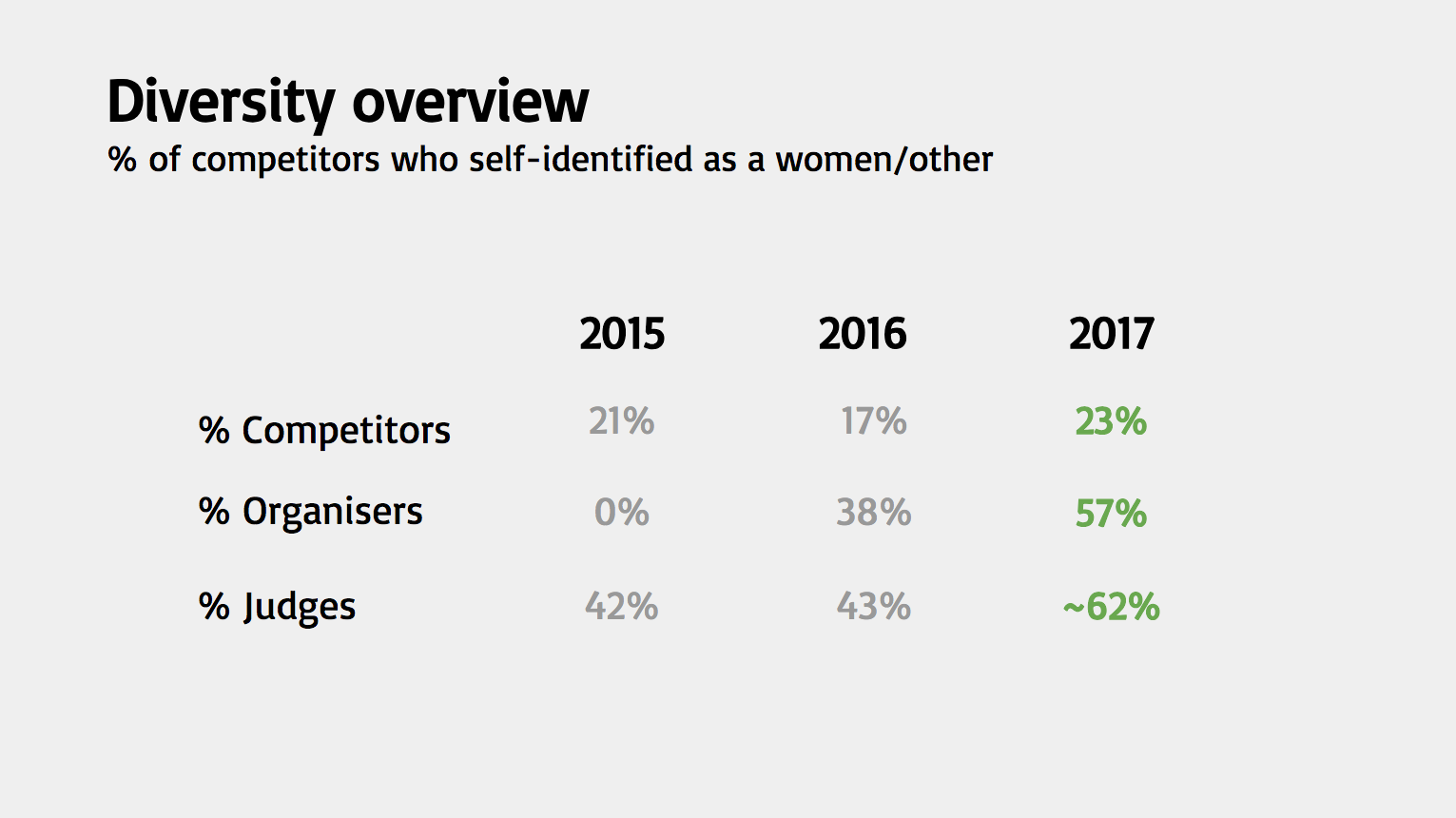
Despite only having information on surface-level diversity, we have piloted a number of initiatives.
Existing pipelines


- Discounted Tickets
We send discounted tickets to groups that focus on diversity in IT. We are keeping this partly to subsidise the financial burden on the student, but also as a buffer on how quickly tickets sell out. There may be students who need more time to think about whether they want to attend or not, and our tickets (especially in Melbourne) sell out quite quickly.


2. Diversity in Judges
Not only do we have judges that correspond to each judging criteria (technical difficulty, business feasibility, creativity, originality), we always make sure to pick judges with a 50–50 gender diversity split (there is also usually an extra judge picked by the headline sponsor, so we don’t have control over that). We also make sure to extend this diversity to race as well.
If you need inspiration for finding a diverse set of speakers/judges/people for your event, look at these lists:
The UNIHACK Judges Twitter List, Women in Tech Twitter List, Google Developer Experts, The Click List, or simply call out on Twitter.


3. Diversity Scholarship
In 2017, we focused on attracting students to UNIHACK, and preparing students who had never attended a hackathon before.
The pipeline for these students after purchasing a ticket were:
- Early access to Slack → Extra tips from organisers
- Early access to Mixer Night → Build familiarity in the community
- Prizes such as GA vouchers and StartupVic membership → Incentive to apply
- SAP Internship Opportunity → Fast track these students into industry
Since 2017, we have interviewed more students (from those who have attended UNIHACK to those who have never attended hackathons before). We found that something we were missing was the continuation of our community from year to year, so we have changed our strategy to focus on that in 2018.
Current focus at UNIHACK
- Attract more participants from diverse and underrepresented backgrounds.
We want to raise the percentage of people who identify as women/other from an average of 20% to 25% by 2019, and reach out to more diversity groups that focus on other underrepresented groups, other than only women in IT.
2. Retain participants from the moment they purchase a ticket until the actual event.
We want to lower the disproportionately higher dropout rates of women, before the hackathon. In Melbourne 2017, out of 118/143 attendees, there was a 14% drop out rate for men and 27% drop out rate for women/other. We are hoping to focus on building a community and outline pipelines for students to feel more comfortable attending a competition alone. We will also be emphasising where students can find team members and socialise with each other earlier on.
Understandably some students see hackathons as an intimidating event (due to perceived lack of skill) or just not a pleasant event (think stinking in a room for 24 hours) — we can promise that UNIHACK is not like that at all.
It’s very important to recognise that diversity in tech initiatives do not aim to vilinise those who are not underrepresented, but rather simply to highlight and to help the underrepresented get up to speed with those who aren’t.
We have decided to establish a commitment to diversity at our hackathon, and will do do our absolute best to play our part.
Thank you to all the people that engaged with us, and let us interview you.
Thank you to the all the people who helped proof read this too!
And thank you to our sponsors, mentors, participants and supporters for allowing us to make this happen.
hackPHS 2019


There's A House Painted Like "Starry Night" In Florida & It's An Enchanting Masterpiece

hackRU 2019


Dynamic locomotion synchronization of bipedal robot and human operator via bilateral feedback teleoperation

https://robotics.sciencemag.org/content/4/35/eaav4282
Abstract
Despite remarkable progress in artificial intelligence, autonomous humanoid robots are still far from matching human-level manipulation and locomotion proficiency in real applications. Proficient robots would be ideal first responders to dangerous scenarios such as natural or man-made disasters. When handling these situations, robots must be capable of navigating highly unstructured terrain and dexterously interacting with objects designed for human workers. To create humanoid machines with human-level motor skills, in this work, we use whole-body teleoperation to leverage human control intelligence to command the locomotion of a bipedal robot. The challenge of this strategy lies in properly mapping human body motion to the machine while simultaneously informing the operator how closely the robot is reproducing the movement. Therefore, we propose a solution for this bilateral feedback policy to control a bipedal robot to take steps, jump, and walk in synchrony with a human operator. Such dynamic synchronization was achieved by (i) scaling the core components of human locomotion data to robot proportions in real time and (ii) applying feedback forces to the operator that are proportional to the relative velocity between human and robot. Human motion was sped up to match a faster robot, or drag was generated to synchronize the operator with a slower robot. Here, we focused on the frontal plane dynamics and stabilized the robot in the sagittal plane using an external gantry. These results represent a fundamental solution to seamlessly combine human innate motor control proficiency with the physical endurance and strength of humanoid robots.
INTRODUCTION
Motivation
State-of-the-art humanoid robots are still unable to match the sophistication and adaptability of human’s innate motor control intelligence. A robotic disaster responder with locomotion and manipulation capabilities similar to those of the average human would be a valuable tool for field applications. If this technology had been available back in March 2011, the catastrophic outcome of the Fukushima Daiichi power plant nuclear disaster could have been vastly mitigated. It is estimated that, if a responder had been able to endure the deadly levels of radiation and enter the facility within the first 24 hours after the cooling system malfunctioned, the first nuclear reactor could have been stabilized (1). However, at the time, no robot of any sort had the autonomy, locomotion, or manipulation capabilities to navigate the unstructured terrain and robustly interact with the environment by opening spring-loaded doors, pushing debris, operating valves, or using tools designed for human workers. Even to this date, in the era of artificial intelligence, programming an autonomous robot to achieve human-level perception and motor control in real environments is extremely challenging and has yet to be demonstrated (2).
Humanoid robots are extremely complex systems that locomote by applying intermittent forces to the environment using contact sequences that must be planned ahead of time using the perceived footholds. These interaction forces often have nontrivial unilaterality constraints (the feet cannot pull on the ground) and are subject to difficult-to-model friction and impact dynamics. In addition, dexterous manipulation requires a whole other level of contact regulation that combines visual, tactile, and proprioceptive perception with the understanding of operation of the object being handled. The controller for an autonomous robot must produce whole-body trajectories that are subject to all these challenges while regulating balance, body momentum, inter-limb coordination, actuation and joint limits, self-collision, external disturbances, and the physical task itself (3). Reliably achieving this level of control sophistication in real-world applications is still an open problem in robotics. On the other hand, humans routinely solve these challenges while continually learning to adapt to unfamiliar scenarios. We envision that this unique human skill can be transferred to a remote robot through whole-body teleoperation. By using the body movement of a human operator to control a humanoid in real time, the machine becomes an equally capable, but expendable, first responder to dangerous situations or remote locations. This solution combines human motor control intelligence with the physical robustness and power density of robots. The key challenge is effectively mapping the human body movement to the robot and intuitively informing the operator about how closely the robot is reproducing the desired motion.
Related work
Motion retargeting from humans to legged machines or animated characters has been an active topic of research for robotics, biomechanics, and computer graphics for many years. Often, during offline retargeting, the operator kinematic data, such as joint angles and center of mass (CoM) trajectory, are measured by a motion capture system (4, 5), and the dynamic data, such as ground contact forces, are estimated by a force plate. Before the target can reproduce the motion, the data are modified to respect the robot’s (or character) physical structure, dynamic characteristics, and limitations. Frequently, this process is performed by an optimizer that approximates the target’s motions to the reference data while maintaining balancing stability (6, 7) or the nuances of the movement of a character (8, 9). This procedure is time insensitive because it is done offline; thus, the complex whole-body trajectory can be extensively refined and the resulting movement reference can be greatly optimized (10). In contrast, online motion retargeting or whole-body teleoperation (11, 12) must provide a feasible reference to the robotic system in real time, making computationally intensive planners prohibitive. In most studies of whole-body teleoperation, the robot’s balancing stability is regulated using a reduced-order model, which guides the motion mapping from the human operator to the robot (13, 14). This model is much simpler than the full-body dynamics but is competent to capture the fundamental properties of the movement that is being mapped. For instance, in the work by Ishiguro et al. (13), the reference motion provided to the robot is obtained by modifying human’s reference using stability considerations from a reduced model, allowing the robot to safely walk. However, human and machine move asynchronously because the operator does not receive any kinesthetic feedback regarding the robot’s relative motion. This unilateral information flow is a common characteristic in all of these studies. The operator commands the robot to move using his/her own body but does not receive any physical information when the robot lags behind, is perturbed, or applies forces to its surroundings.
We argue, however, that when dynamically interacting with the environment, humans heavily rely on the feedback forces from their motor actions (15). They use this kinesthetic feedback to learn how to cope with the added dynamics and to create muscle memory for recurrent behaviors. For instance, when a firefighter uses his/her entire body to push a heavy door, the subsequent motion is completely different if the door turns out to be locked or if it is free to open. Following this rationale, the teleoperated robotic responder must provide the operator with physical feedback from its actions such that the operator can intuitively use innate motor intelligence to plan the movement effectively. Thus, unilateral teleoperation strategies are unlikely to be successful in unpredictable real scenarios unless the robot has a nontrivial degree of autonomy to overwrite infeasible or erroneous commands. Yet, to the best of our knowledge, in very few studies in the literature was the operator provided with kinesthetic body feedback from the machine’s motion during teleoperation. In previous studies, forces were applied to the operator’s torso as an attempt to inform about the robot’s semistatic stability condition (16). A similar strategy using vibro-tactile feedback has also been adopted (17). However, in both studies, the machine could only perform slow movements on flat ground, and it is unclear how to extend these strategies to agile locomotion, such as walking or jumping, limiting their usefulness for real applications. In contrast, dynamic teleoperation with bilateral feedback of robotic manipulators is a well-studied research topic (18, 19). But fixed-base manipulators can apply arbitrarily large forces to their surrounding without regulating balance and step placement, differently from the top-heavy and mobile humanoid robots. Thus, existing bilateral feedback strategies used for robotic arms are not directly applicable to whole-body teleoperation of legged robots.
To address these research challenges, this paper describes a teleoperation system, shown in Fig. 1, and a control strategy to dynamically synchronize the lower-body motion of a human operator and that of a bipedal robot. Through this virtual coupling, operator and robot can simultaneously take steps, jump, and walk. The core components of human locomotion are scaled to the bipedal robot using a simplified model for legged dynamics, the linear inverted pendulum (LIP). Simultaneously, the same model is used to compute feedback forces that are applied to the waist of the operator, near the CoM, to match the operator motion velocity to that of the robot. If the robot moves faster, the human-machine interface (HMI) applies a force to speed up the translation of the operator’s CoM. If the robot lags behind, the HMI simulates drag to slow down human movement. Hence, the feedback force informs the operator about how closely the robot is reproducing human motion in real time. To focus the analysis and simplify the balancing task, we stabilized the robot in the sagittal plane using an external gantry, preventing it from falling forward or backward. However, the gantry did not provide any support in the frontal plane, and we assumed that the controllers for both these planes can be decoupled.

(A) The human operator controls the small bipedal robot, Little HERMES, to take steps in place. (B) The core components of the locomotion dynamics are mapped from operator to the robot using a simplified model, the LIP. Simultaneously, a feedback force [red arrows in (B1) and (B2)] is applied to the torso of the operator, near the CoM, to synchronize the motion of operator and robot. This feedback force is proportional to the relative instantaneous velocity between the operator and robot. (C) The machine uses human reference to reproduce stepping motions in real time.
Model reduction: The LIP
Because of the complexity of the legged systems and the intricacy of walking mechanics (nonlinear, hybrid, and underactuated dynamics), researchers often approximate particular locomotive behaviors using simplified models. These models must capture the principal components of the full system dynamics while remaining tractable. A common strategy is to use the insights obtained from the reduced models to develop intuitive heuristics that govern the high-level controller of legged robots (20). The LIP is a powerful one-dimensional (1D) model popularly used to capture the fundamental dynamics of the CoM of bipedal systems during upright balancing and walking (14). The second-order equation of motion of the LIP describes the unstable behavior of the CoM of the system with respect to its center of pressure (CoP): the point on the ground from where a single force vector originates and summarizes the net effect of all the contact forces applied to the feet (21). By regulating the contact forces between each foot and the ground, the position of the CoP is manipulated within the area that spans the supporting feet. Movie 1 illustrates this model simplification, which is also adopted in our previous work (22). The CoP position pH(t) represents the input to the LIP equation of motion that approximates the horizontal displacement xH(t) of the human CoM
x¨H(t)=ω2H(xH(t)−pH(t))
(1)where x¨H(t) is the horizontal acceleration of the CoM and ωH is the constant natural frequency of the pendulum, which dictates how fast it falls. This linear equation models the upright unstable dynamics of the bipedal system, in which the CoM naturally accelerates away from the CoP. For example, concentrating the ground contact forces under the heels causes the body to lean and later fall forward. In this model, the CoM can be actively stabilized and manipulated by properly positioning the CoP.
Movie 1. Summary of the bilateral teleoperation strategy adopted in this work.
Previous work (23–25) demonstrated that, instead of individually controlling the CoM position and velocity [xH(t) and ẋ H(t)], it is sufficient to regulate the unstable component of the LIP dynamics to balance and walk. This fundamental component associated with the unstable LIP behavior is a composite state given by the horizontal CoM position and its normalized velocity
ξH(t)=xH(t)+ẋ H(t)ωH
(2)
The state ξH(t) is named the divergent component of motion (DCM) and has been extensively used for controlling the locomotion of bipedal robots. Beyond the field of robotics, biomechanics studies have also presented compelling evidence that suggests that humans regulate a linear combination of the CoM position and its velocity, similar to the DCM, to walk and react to external disturbances (26). These studies evidence the importance of the interplay between the DCM and the CoP for dynamic legged locomotion. Inspired by this observation, we assumed that the operator stably manipulates the DCM during locomotion by shifting the position of the CoP on the ground. To command the robot to simultaneously perform the same feat, we provided a motion reference to the machine by scaling the position of the human DCM and CoP. Because the human and the robot often have substantially different physical properties, we performed this transformation using similarity analysis.
Similarity of dynamic systems
Similarity analysis of dynamic systems has often been used for the comparison of animal movements across markedly different physical scales (27, 28). For instance, one can compare the locomotion performance of a cheetah with that of a cockroach by normalizing their running speeds by their respective body lengths. By this principle, systems are geometrically similar when they have the same shape, but the dimensions are scaled by some constant factor. Two motions are kinematically similar if time is scaled by a constant number and dynamically similar if all forces follow a constant ratio. Dimensional analysis of the equations that describe the mathematical models enables the comparison of systems that have different physical or temporal characteristics. To illustrate this procedure, researchers have performed dimensional analysis of the LIP to derive the equation of motion for a dimensionless model (29). With this generalization, the fundamental behavior of the LIP was analyzed independently of particular parameters, and the motions of pendula with different lengths (or inertias) were shown to be dynamically similar.
The present work leverages this idea: We aimed to make the simplified robot dynamics similar to those of the human-reduced model via teleoperation. In essence, the robot movement ideally reproduces DCM and CoP trajectories similar to those of the operator. Hence, the motion reference mapped from human to robot and the feedback force applied to the operator were designed to guarantee this dynamic similarity. When we normalized the DCM and CoP positions using constant parameters of each system, we obtained states that ideally follow identical dimensionless trajectories, independent of scale. In the present work, horizontal states, such as the DCM and CoP, were normalized using the nominal distance between the feet (dH and dR) and vertical states using the nominal CoM height (hH and hR). Subscripts “H” and “R” indicate “human” and “robot,” respectively. States with an apostrophe indicate dimensionless values [for instance, x′R(t)=xR(t)dR]. Figure 2 illustrates the condition of dynamic similarity that our teleoperation strategy aims to achieve.

In the ideal scenario, the horizontal motion of the robot DCM [ξR(t)=xR(t)+ẋ R(t)ωR] and CoP pR are dynamically similar to those of the human operator, which means that their dimensionless trajectories match [ξ′H(t)=ξ′R(t) and p′H(t)=p′R(t)]. The CoMs are not required to coincide because manipulating the DCM is sufficient to control locomotion. Time dependency of the state variables is omitted for clarity.
Manuscript context and contribution
This work builds on promising results for upper-body teleoperation of highly dynamic physical interactions achieved by the HERMES humanoid robot (30). Here, we complement our previous work and present a fundamental solution to dynamically synchronize the locomotion of the bipedal robot to that of the human operator. To achieve this goal, we used bilateral feedback to impose the dynamic similarity between the reduced models for the robot and that of the operator. With this virtual constraint, the operator could generate, in real time, lower-body trajectories that were dynamically compatible with the robot’s geometric, inertial, and temporal properties. To experimentally demonstrate this strategy, we developed a wearable HMI, named the balance feedback interface (BFI), and a small-scale bipedal robot, named Little HERMES (31). This work focused on studying fundamental locomotive skills such as synchronous stepping, jumping, and walking via teleoperation. Instead of being preprogrammed trajectories that the robot simply replay, these coordinated dynamic motions were induced by the operator in real time through the BFI.
RESULTS
Similarity-based bilateral feedback teleoperation
To evaluate our teleoperation strategy, we used Little HERMES, a small-scale machine with physical properties substantially different from those of a human adult. These include (i) smaller total mass (mR = 6 kg) and inertial distribution, (ii) shorter nominal CoM height (hR = 35 cm), and (iii) shorter nominal distance between the feet (dR = 25 cm). It is intuitive that a short pendulum has a faster oscillation period than a longer one. Analogously, a smaller-scale robot has a faster natural frequency and, consequently, a faster stepping frequency. We used bilateral teleoperation to allow a human operator to control this machine despite dissimilar physical properties. The forward path (human to robot) of the teleoperation feedback sends the human DCM and CoP normalized positions to the robot to reproduce. The robot controller commands a motion that achieves the similarity ξ′R(t)=ξ′H(t) and p′R(t)=p′H(t) simultaneously. However, the time rate of change of the DCM is bounded by the natural frequency of the system: A pendulum cannot fall faster than its natural dynamics allows. To ensure that human and robot DCMs will evolve similarly in time, the backward path (robot to human) of the bilateral teleoperation consists of a horizontal force applied to the CoM of the operator that is proportional to the dimensionless velocity error
FBFI(t)=kH(ẋ ′R(t)−ẋ ′H(t))
(3)
This equation indicates that if the robot moves (falls) faster than the operator (∣ẋ ′R∣>∣ẋ ′H∣), the force feedback will push the operator to move faster. If the robot lags behind (∣ẋ ′R∣<∣ẋ ′H∣), the force feedback applied to the operator will create the effect of drag and slow down human motion. The constant gain kH maps the dimensionless velocity error to human mass and height proportions. This means that a heavier or taller operator will experience proportionally scaled feedback forces for the same relative motion error. The derivation of this expression is presented in Materials and Methods and in previous work (32). Movie 1 summarizes the bilateral teleoperation strategy.
Dynamic stepping in place
During teleoperation, the controller of the robot commands its CoP position on the ground to match the human reference by regulating the contact forces under each foot. When both feet exert nonzero forces (double support), the CoP is located at an intermediate point between its feet, and the dimensionless CoP is within the interval −0.5<p′R<0.5. When, for instance, the CoP is shifted to the right foot, as indicated by the magenta regions in Fig. 3B, it indicates that the left foot has lost contact and exerts zero force (p′R=0.5). When the robot controller detects this condition, it commands its left foot to follow a swing trajectory similar to that of the operator’s left foot. An analogous situation occurs when the CoP is shifted to the left foot instead, in which p′R=−0.5, and represented by green regions on Fig. 3B. These support transitions are further detailed in fig. S1. Stepping in place consists of a coordinated sequence of right and left feet support and swing as depicted in Fig. 3. Figure 3A displays the time evolution of the human and robot dimensionless DCM trajectory, and Fig. 3B shows the relative CoP trajectory. In addition, the feedback force FBFI(t) produced by the BFI, and applied to the CoM of the operator, is shown in Fig. 3C. This experiment is illustrated in movie S1. The vertical swing foot trajectory of the robot and the operator for several steps is displayed in fig. S2.

Dynamic synchronization of human and robot DCM and CoP, the two fundamental components of the LIP. (A) Comparison between human and robot DCM normalized by the distance between the feet dH and dR. The high-frequency component of the robot DCM is an artifact of the foot compliance. (B) Dimensionless CoP position for the operator (blue) and the robot (red). The areas shaded in magenta indicate right foot support, as illustrated by the cartoon in the magenta box, when the relative CoP trajectory is flat at p′R=0.5. Left foot support is analogously represented by green shaded areas and the cartoon in the green box (p′R=−0.5). The cartoons also illustrate the robot swing foot trajectory δR(t) scaled from the human reference δH(t) and the feedback force FBFI(t) in red. (C) Time evolution of the feedback force FBFI(t) applied to the CoM of the operator during teleoperation.
Additional experiments are presented in the Supplementary Materials. Figure S3 depicts a trial in which the operator commands the robot to move right to left in the frontal plane without taking steps (always double support). Human and robot DCM and CoP matched closely. The synchronization effect of the feedback force FBFI(t) is revealed in fig. S4. In this case, the feedback force was initially set to zero and subsequently enabled at about 3.5 s after the start of the experiment. The feedback force stabilized the robot DCM. Last, movie S2 depicts the ability of the robot controller to regulate the contact forces with the ground. In this experiment, an autonomous controller based on the LIP regulated the position of the CoP to maintain the DCM at the midpoint between the feet in the absence of an operator.
Dynamic walking
Forward propulsion occurs when the stance foot applies a tangential contact force against the ground in the anteroposterior direction during single support. In addition, the magnitude of this force in coordination with the appropriate stride length regulates the walking speed (29). Using this heuristic, the operator can generate a reference propulsive force by, for instance, leaning against a resistive string and taking steps in place, as demonstrated in Fig. 4A. For this experiment, the external gantry stabilizes the robot yaw (craniocaudal axis) and pitch (left-right axis) rotation, as illustrated in fig. S5B. While in single support, the stance foot of the robot applies a tangential ground contact force proportional to the reference provided by the operator and given by
FyR(t)=αFyH(t)
(4)which modulates forward walking. In addition, the horizontal step length is regulated proportionally to the walking speed: The faster the robot walks, the longer the stride is. If α is defined negative, the robot walks backward, as shown in movie S3. We envision that this strategy can be further extended to more complex behaviors such as turning and running, which is the topic of future work.

(A) Operator commands the robot to walk by stepping in place while leaning forward and applying a static force against a string. The robot produces a similar tangential force with the stance foot, propelling the machine forward. Walking speed ẏ R is controlled by the tangential ground contact force FyR in combination with the proper stride length δyR. (B) Robot jumps by modulating the magnitude of the net contact force similarly to the operator. (B1) to (B3) illustrate this procedure and are indicated by the vertical yellow, green, and magenta lines in (B4) and (B5). (B4) Dimensionless vertical component of the net contact forces from the operator and robot. (B5) Vertical displacement of the CoM estimated from leg kinematics and from the external gantry.
Jumping
The CoP is defined as the point on the ground where an equivalent net force originates and summarizes the effect of all the contact forces applied to the body. As described by the LIP model, the horizontal position of the CoP is used to maintain balance and take steps. In addition to its location, the operator also modulates the magnitude of this net contact force to regulate the CoM height. This magnitude is normalized by the total body mass mH of the operator and transmitted as reference to the bipedal robot. The machine produces a net contact force with similar magnitude to that of the operator. With this control authority, the human can command the robot to produce an upward thrust large enough to leave the ground. Figure 4 (B1 to B3) shows instances of a teleoperated jump. Figure 4B4 depicts the dimensionless reference net force FzHmHg measured by the force plate and normalized by human mass. The net vertical force produced by the robot, represented by the dimensionless quantity FzRmRg, is also shown. Figure 4B5 displays the CoM height of the robot estimated from leg kinematics zlegR in cyan and measured using the external gantry zgantryR in black. When the robot is airborne, the height estimation from leg kinematics saturates at maximum leg extension. The teleoperation of consecutive jumps is shown in movie S4.
DISCUSSION
Our research focuses on creating a teleoperation system that enables a human to intuitively control the movement of a humanoid robot while receiving kinesthetic feedback related to the motion of the robot. When synchronized with the remote robot, the operator generated stepping and walking references that were dynamically feasible for the machine to reproduce. Ideally, this teleoperation strategy eliminates the necessity for task-specific and computationally hungry perception and whole-body motion planning algorithms typically used by autonomous machines (24, 33). In this work, we focused on a fundamental locomotion synchronization strategy. This teleoperation strategy is demonstrated via three representative experiments: (i) stepping in place, (ii) walking, and (iii) jumping. Stepping illustrates the control of the fundamental balancing and locomotion mechanism. It is achieved by coordinating the interplay between the DCM and the CoP trajectories, in addition to controlling the swing leg motion and the feet placement. These are essential components required for agile locomotion in unstructured terrain. Dynamic synchronization is revealed by the point-foot design of the bipedal robot: The machine is unstable in the static sense during single support. To illustrate this scenario, movie S5 demonstrates several unsuccessful early attempts to take steps. Walking extends the basic stepping-in-place behavior to demonstrate how the operator can regulate the locomotion of the robot. Similar strategies can be used to extend this capability to other locomotive actions such as running and turning. Last, jumping exemplifies the ability to generate large contact forces and to deal with impacts. We envision that the ability to aggressively push against the ground and accelerate the body upward can be extrapolated to whole-body manipulation tasks that require regulation of large contact forces such as pushing or lifting heavy objects.
We assume that the motion error evident in Fig. 3 (A and B) originates largely from (i) the mechanical properties of the foot sensor material and (ii) the point contact of the spherical foot. The foot sensor underdamps the vibrations caused by unmodeled impacts with the ground, causing the entire robot to shake momentarily and introducing noise in the velocity estimation (and consequently the DCM). This can be evidenced when comparing Fig. 3A with the first 4 s of fig. S3A, when there were no impacts, and the motion error was very small. Selecting a different material with improved damping properties for the foot sensor will likely reduce this issue. The effect of the foot compliance is also evident in the high frequency ringing in Fig. 4B4. The DCM tracking performance is further degraded during single support or at large amplitudes of the CoP trajectories, which is demonstrated by comparing the first and second halves of fig. S3. We assume that the lack of ankle supination or pronation torque prevents fine regulation of the robot CoP when standing on one of the feet. Because of this degradation in control authority, the robot motion briefly lags the operator reference. The addition of a more substantial foot and the utilization of balancing strategies that use angular momentum regulation (29) could help mitigate this problem. Last, it is difficult to define the acceptable tracking error that can be tolerated for successful synchronization largely due to the uncertainties introduced by the human. It is likely that the expertise of the operator heavily affects how limitations of the system are anticipated and compensated for.
Limitations of the approach
This pilot study is based on a planar linear model with limited dynamics. In addition, the robot is not designed to balance in the sagittal plane without the gantry due to the simplicity of the leg design and the point-contact feet. Future implementation of more complex 3D motions, such as running and turning, will require more sophisticated model and machine (34) and is a topic of future work. However, the fundamental idea of dynamic similarity presented in this work should be preserved even for complex systems. Another limitation of the present study originates from the exclusively horizontal force feedback, FBFI, applied to the operator. We assume that including additional kinesthetic feedback for total angular momentum, for instance, will enable the utilization of strategies based on reactive inertia, such as the “hip strategy,” for balancing or absorbing external disturbances (35, 36).
In addition, an evident drawback of our method relates to a notorious issue of telerobotics: communication delay. This issue becomes even more pertinent for time-sensitive occasions, such as during highly dynamic motions. Although not within the scope of the present study, it is still unclear how much delay the strategy proposed in this paper can tolerate. However, given the relatively slow natural frequency of the legged systems in this work, we expect that the bilateral teleoperation will still be successful for moderate amounts of communication lag. In addition, we argue that the challenge of achieving high-speed remote communication stands in a considerably shorter technological horizon than achieving reliable human-level perception and motor control for autonomous robots. Thus, we believe that bilateral feedback teleoperation stands as a promising shorter-term solution for deploying robots to real applications.
Future work
The goal of our strategy is to transfer the burden of perception of the surroundings and the motion planning to the human, considerably reducing the autonomy requirements for the robot. We assume that, with sufficient training, the operator will learn how to naturally cope with the robot-added dynamics. Using the kinesthetic feedback, the experienced operator should develop the “muscle memory” to effectively control the machine. This adaptation to dynamic conditions has been demonstrated for simple dynamic systems (37). We assume that this operator will be able to adapt to unfamiliar scenarios and improvise motions that the machine has not performed beforehand—a fundamental human skill and a capability still far from being achieved by autonomous machines. Future work includes an evaluation of the learning rate for inexperienced operators and the definition of training procedures to improve the synergy between human and robot. We would like to explore how human intention can be anticipated using other biosignals, such as gaze tracking, electromyography, and electroencephalography. Last, on the human side, we will look into the trade-offs between the required feedback (kinesthetic, visual, auditory, etc.) to the operator and their associated cognitive load, especially for long periods of operation.
We envision that a robotic disaster response robot will seamlessly combine the power density of machines with the control skills of humans to perform highly demanding physical tasks. Toward this vision, the control architecture presented in this work introduces fundamental ingredients to dynamically couple the operator to the humanoid robot. Our future research will focus on combining the manipulation performance demonstrated by HERMES (38) with the locomotion control introduced here by Little HERMES. For instance, a disaster responder would use these combined abilities by taking steps to build up momentum and to subsequently dump that energy to break down a blocked door, as shown in Fig. 5. Future work will address several core challenges to create a capable humanoid disaster responder. These challenges include the development of a generalized teleoperation strategy for 3D motion in parallel with a legged robot capable of balancing itself without the gantry. At that point, we must prescribe the boundaries of human-robot shared autonomy, which is defining the extent to which the robot follows human motion or makes autonomous decisions to modify suboptimal, conflicting, or erroneous commands that may jeopardize stability or the completion of the task at hand.

We intend to combine previous results for manipulation, enabled by HERMES, and locomotion, introduced here by Little HERMES, to develop a capable robotic responder. This robot will leverage human motor control and perception skills to perform physically demanding tasks that require whole-body coordination in addition to balance regulation.
Last, the method presented here could also be further explored under the lights of motor rehabilitation. For such application, we envision that the physiotherapist could provide intuitive physical cues and support for gait rehabilitation through the BFI by “teleoperating” a patient connected to a second BFI. Both individuals would become more synchronized as the patient walking performance improves with treatment. In addition, the kinesthetic feedback to the physiotherapist could potentially provide valuable information about the impairment condition of a particular patient.
MATERIALS AND METHODS
The proposed teleoperation system requires three major components: (i) the bipedal robot, (ii) the BFI and operator, and (iii) the bilateral feedback teleoperation law. First, we describe the bipedal robot developed by our group, highlighting design features that enable proper force control and agility for legged locomotion. Next, we describe the design of the BFI for high-speed motion capture and kinesthetic body feedback. Last, we derive the bilateral feedback law that maps the information between the operator and the remote robot. We briefly describe the controller of the robot here, and the reader can find further information in our previous work (31, 32). The experiments presented here were conducted with a single experienced operator. The data for the experiments were collected after the operator became familiar with the system; at that point, each experiment was conducted a single time. Emergency stops were included to shut off the BFI or the robot in case of failure or danger.
The bipedal robot: Little HERMES
The experiments presented in this paper were conducted with Little HERMES (31), shown in Fig. 6, a small-scale bipedal robot with three degree-of-freedom (DoF) legs and point feet. During the stepping in place and jumping experiments, a boom with a spherical base joint constrained the robot to move in its frontal plane. For the constrained walking experiment, a passive linkage structure stabilized the robot yaw and pitch rotation but allowed the robot to translate in the anteroposterior direction. Both gantries are shown in fig. S5.

The design of the small-scale robot is based on principles specific for agile legged locomotion. (A) Custom actuators were designed for impact mitigation and high-bandwidth torque control. (B) Lightweight limbs have negligible inertia and allow fast leg swing. A timing belt transmits the torque to the knee joint from the motor mounted coaxial to the hip axis. (C) Impact-robust and lightweight foot sensors measure three-axis contact forces and were used as contact switches. (D) A ruggedized IMU estimates the robot’s torso posture, angular rate, and linear acceleration at 250 Hz. (E) Real-time computer sbRIO 9606 from National Instruments controls the robot at 600 Hz. (F) The robot is powered by two three-cell lithium-polymer batteries in series. (G) A rigid and lightweight frame minimizes the robot mass.
Little HERMES uses a number of design principles that allow contact force regulation at high bandwidth. Each leg has three DoFs: hip ab/adduction, hip flexion/extension, and knee flexion/extension. The actuators were designed from off-the-shelf gimbal motors with a custom single-stage 6:1 planetary gearbox and an integrated current-control driver with energy regeneration (39). An efficient 1.6:1 timing belt transmission connects the knee joint to its actuator, mounted proximal to the body and coaxial with the hip flexion/extension actuator. These features were combined with the lightweight leg design (together about 10% body mass) to minimize energy losses from frictional and inertial forces. These features enabled high-bandwidth force control from motor current and leg kinematics alone, without requiring springs or force/torque sensors (31, 40).
Custom foot sensors monitored the contact forces with the ground. We used these sensors to estimate the robot CoP and as contact switches but not for closed-loop contact force control. As shown in fig. S6, these lightweight devices (about 50 g each) can measure three-axis forces and are composed of an array of four piezoresistive sensors that are loaded by the deformation of a urethane hemisphere during interaction with the ground (41). These impact-robust and lightweight sensors are more appropriate for legged locomotion than conventional stiff, heavy, and bulky load cells or force/torque sensors. In addition, the polymeric deformable material could be designed to have stiffness and damping properties tuned to the application. We found the material used for our sensors to be excessively springy and intend to replace it with polymers with improved dampening characteristics, such as sorbothane. Figure S7 illustrates the open-loop contact force control performed by the bipedal robot.
The embedded real-time computer, an sbRIO 9606 from National Instruments, runs the robot control loop at 600 Hz. It communicates with the actuators via a dual-channel high-speed CAN bus card NI9853 and with the feet sensors with an analog input card NI9205. The IMU, VectorNav VN-100, provides body orientation and angular rates at 250 Hz. Two three-cell lithium-polymer Venom batteries in series power the entire robot.
The BFI and human operator
Human motion data were collected by the BFI, a highly backdrivable HMI designed to be transparent to the user and shown in Fig. 7. This high-speed motion capture system used 12-bit encoders to measure human torso position and orientation in space (five DoFs, no torso yaw). The three-DoF spatial position of the feet was estimated using two passive arms connected to the operator’s feet. The BFI can apply large horizontal feedback forces (up to 100 N) to the operator’s waist, near the CoM. The feedback force and torso posture tracking were performed by two actuation modules, each with three DoFs (one actuated and two passive), as depicted in Fig. 7A. The torso posture was estimated by solving the forward kinematic of both modules together. The desired feedback force FBFI was achieved by coordinating the force produced by the both actuation modules. Figure S8 shows the force control performance for one of the stepping-in-place teleoperation experiments. A six-axis force plate captures the human CoP and the normal and tangent components of the ground contact forces that the operator applies during motion. The real-time computer, a cRIO9082 from National Instruments, ran the control loop and estimated human posture at 1 kHz. The communication rate with the robot was also performed at 1 kHz.

(A) Custom HMI was designed to be transparent to the operator and to capture human motion data at high speed (1 kHz). (B) BFI has two underactuated modules that together track the position and orientation of the torso and apply forces to the operator’s CoM. (C) Each actuation module has three DoFs, one of which is a push/pull rod actuated by a DC brushless motor (Maxon EC90 Flat). A pair of load cells measures the actual forces applied to the operator. These sensors were not used for closed-loop force control. Force control was achieved via current-based torque control of the motors. (D) A series of linkages with passive joints were connected to the operator’s feet and track their spatial translation. (E) Real-time controller cRIO 9082 from National Instruments closed the BFI control loop and sampled data at 1 kHz. (F) A 3 feet–by–3 feet force plate estimated the operator’s CoP position and measured the shear and normal components of the operator’s net contact force.
Bilateral feedback teleoperation law
During teleoperation, the robot reproduces human motion by tracking reference DCM and CoP trajectories. To achieve this, the controller of the robot computes two components of the net horizontal force applied by both legs together to the CoM: (i) FrefxR(t) is a feedforward term calculated by scaling the human ground contact force and (ii) FerrorxR(t) is responsible for stabilizing the motion and compensating for tracking errors from the desired DCM reference. The linear compensation uses a constant gain Kx. With these two components, the horizontal equation of motion for the CoM of the robot is given by
mRx¨R(t)=FrefxR(t)+FerrorxR(t)
(5)or
mRx¨R(t)=FrefxR(t)+Kx(ξxH(t)dH−ξxR(t)dR)
(6)
The net horizontal force applied to the CoM of the operator has two terms: (i) FxH(t) is the horizontal component of the contact force that the operator generates against the force plate and (ii) FBFI(t) is the feedback force applied by the BFI. The horizontal equation of motion for the human CoM is given by
mHx¨H(t)=FxH(t)+FBFI(t)
(7)
To derive the expressions for the feedforward term FrefxR(t) and the feedback force FBFI(t), we use the desired CoP similarity
pR(t)dR=pH(t)dH
(8)and the CoP Eq. 1 to obtain
xR(t)dR−x¨R(t)dRω2R=xHdH−x¨H(t)dHω2H
(9)
If we assume that the robot reproduces human DCM reference (ξ(t)dR=ξH(t)dH or FerrorxR=0), we use Eqs. 6 and 7 to write
ẋ R(t)dRωR+FrefxR(t)mRdRω2R=ẋ HdHωH+FxH(t)+FBFI(t)mHdHω2H
(10)
The expressions for the feedforward term and the feedback force are computed by satisfying the equality (Eq. 10). The law that scales the operator contact force to provide a feedforward term for the robot controller is given by
FrefxR(t)=mRdRω2RmHdHω2HFxH(t)
(11)
The force feedback that is applied to the operator is defined by
FBFI(t)=mHdHω2H(ẋ R(t)dRωR−ẋ H(t)dHωH)
(12)
From the desired net contact force to be applied to the CoM, the robot controller computes the individual force contribution for each foot. In this work, this force distribution problem is performed by solving a linear system (31). For more complex robots, this problem is commonly addressed by an optimization-based solver, often formulated as a quadratic program (3, 25). A detailed analysis of this bilateral feedback law was done in our previous work (32).
The high-level control loop of the system is depicted in Fig. 8. First, human motion information is transformed into reference for the robot using a reduced model, the LIP. Next, the robot controller uses this reference to compute the desired ground contact forces for the right and left feet. The “tracking correction” block describes the stabilizing equation for FerrorxR(t). Last, the BFI applies a feedback force to the operator that is proportional to the dimensionless relative velocity of human and robot CoM, according to Eq. 12.

Human kinematic and dynamic data on the far left were transformed into a reference for the robot using the reduced model, the LIP. This transformation computed the desired DCM state ξ′H and the appropriate contact forces FrefxR and FrefzR that the robot must apply to the ground to reproduce human motion. With this information, the robot-embedded controller computed the required contact force to be applied by each foot. The feedback FBFI applied to the operator is proportional to the relative motion velocity between operator and robot.
When one of the robot feet loses contact with the ground, it follows the trajectory of the swing foot of the operator. The desired Cartesian deviation δR(t) from the nominal stance is computed by scaling the operator foot deviation δH(t) from nominal stance. During right leg stance, for instance, the desired left foot swing trajectory follows the deviation from nominal stance given by
δR(t)=⎡⎣⎢⎢δxR(t)δzR(t)⎤⎦⎥⎥=⎡⎣⎢⎢dRdHδxH(t)hRhHδzH(t)⎤⎦⎥⎥
(13)
SUPPLEMENTARY MATERIALS
robotics.sciencemag.org/cgi/content/full/4/35/eaav4282/DC1
Fig. S1. Stances during teleoperation.
Fig. S2. Swing foot vertical trajectory.
Fig. S3. Right-to-left motion teleoperation via bilateral feedback.
Fig. S4. Motion synchronization using force feedback.
Fig. S5. Gantries used to constrain the robot during experiments.
Fig. S6. Soft force sensors used for the robot feet.
Fig. S7. Bipedal robot contact force control.
Fig. S8. BFI force control.
Movie S1. Teleoperation of stepping in place.
Movie S2. Robot autonomous balancing controller.
Movie S3. Teleoperation of constrained walking.
Movie S4. Teleoperation of consecutive jumps.
Movie S5. Compilation of unsuccessful stepping experiments.
http://www.sciencemag.org/about/science-licenses-journal-article-reuse
This is an article distributed under the terms of the Science Journals Default License.
REFERENCES AND NOTES
Acknowledgments: We would like to thank B. Katz for designing the actuators used in the robot and M.Y. (Michael) Chuah for the help manufacturing the foot sensor. We would also like to thank A. Wang and P. Wensing for the insightful discussions about the ideas presented here. Funding: This work was supported by Hon Hai Precision Industry Co. Ltd. via award ID no. 025885 and Naver Labs Corporation via award ID no. 026921. Author contributions: J.R. proposed and tested all the theoretical contributions for bilateral teleoperation presented in this work, including modeling, control, and simulation. J.R. conceptualized, designed, and manufactured the HMI and the bipedal robot Little HERMES, except for the actuators. S.K. proposed the initial concept for whole-body teleoperation, was the supervisor for the project, and provided the overall research direction and funding. Competing interests: The authors declare that they have no competing financial interests. Data and materials availability: All data needed to evaluate the conclusions in the paper are present in the paper or the Supplementary Materials.
- Copyright © 2019 The Authors, some rights reserved; exclusive licensee American Association for the Advancement of Science. No claim to original U.S. Government Works
Hurricanes Spiraling
Ynés Mexía: 5 Fast Facts You Need to Know
Our greatest glory

What is a Fourier Series? (Explained by drawing circles) - Smarter Every Day 205
You won't believe your eyes
Want to tweet this? Click here: http://bit.ly/1MI4z9L
Click here if you're interested in subscribing: http://bit.ly/Subscribe2SED
If you like to support Smarter Every Day via the sponsor go for it at http://www.Lynda.com/Smarter
Check out Greg's page at: http://www.ohmbrew.net
More info! ⇊ Click below for more links! ⇊
Check out Greg's page at: http://www.ohmbrew.net (HE HAS SCHEMATICS!)
Tweet This Video: http://bit.ly/1MI4z9L
Smarter Every Day Instagram: http://instagram.com/smartereveryday Patreon Support Link: http://www.patreon.com/smartereveryday Twitter: http://twitter.com/smartereveryday www.facebook.com/SmarterEveryDay
Ambiance and musicy things by: Gordon McGladdery did all of the sound design for the video. http://ashellinthepit.bandcamp.com/
A special thank you to Dr. Stuart Anstis. http://anstislab.ucsd.edu/
Read some of Dr. Anstis's Papers: ~~~~~~~~~~~~~~~~~~~~~~~~~~~~
Tweet ideas to me @SmarterEveryDay
Instead of saving for my kids' college, I make videos using the money I would have saved. The thought is it will help educate the world as a whole, and one day generate enough revenue to pay for their education. Until then if you appreciate what you've learned in this video and the effort that went in to it, please SHARE THE VIDEO!
If you REALLY liked it, feel free to pitch a few dollars towards their college fund by clicking here: http://bit.ly/KidsCollege Warm Regards, Destin
Caption authors (French)
Banane ApocalyptiqueArise TreflesBurningbeats soundJonathan Dubé
Caption authors (Norwegian)
Caption author (Chinese (Taiwan))
Caption authors (Bulgarian)
State-of-the-art CapitalGeorgi Zahov
Caption author (Hindi)
Caption authors (Arabic)
Seif EddinedloooolAbdelrazik HarbArab Mohammad
Caption authors (German)
Category
How to make a laser security alarm system
Astronauts in Space 'Feel the Power' of Hurricane Dorian as NASA's Florida Spaceport Braces for the Storm
Update for Sept. 3: As of 5 a.m. EDT, Hurricane Dorian has weakened to a Category 3 storm.
As Hurricane Dorian churned across the Bahamas Monday (Sept. 2), the storm's awed astronauts in orbit with its raw power and set NASA's Kennedy Space Center in Florida on high alert for potential damage.
As of 11 p.m. EDT (0200 GMT), Dorian was stalled just north of Grand Bahama Island as the Category 4 storm battered the island with maximum sustained winds of nearly 130 mph (215 km/h), according to a National Hurricane Center update. Earlier Monday, the storm was hard to miss to astronauts looking down on Earth from the International Space Station.
"You can feel the power of the storm when you stare into its eye from above," NASA astronaut Nick Hague wrote on Twitter while sharing a striking photo of the storm. "Stay safe everyone!"
Video: Here's the Latest Video of Hurricane Dorian from Space
Watch: See Hurricane Dorian in Action in these Gifs from Space

NASA astronaut Nick Hague of the Expedition 60 crew snapped this photo of the eye of Hurricane Dorian, a Category 4 storm, from the International Space Station on Sept. 2, 2019 as the storm stalled over the northern Bahamas.
(Image credit: Christina Koch/NASA via Twitter)
Hague's crewmate Christina Koch, also of NASA, snapped several more views of Dorian as the space station flew 260 miles (418 kilometers) overheard. Her four-photo series reveals the storm's eye up close, as well as views of the entire hurricane as it crossed the northwestern Bahamas.
"Hurricane Dorian as seen from Space Station earlier today," Koch wrote on Twitter. "Hoping everyone in its path stays safe."

NASA astronaut Christina Koch of the Expedition 60 crew snapped this photo, one in a series, from the International Space Station on Sept. 2, 2019 as the storm battered the northern Bahamas. The storm's eye is clearly visible in this close view.
(Image credit: Christina Koch/NASA via Twitter)

The scale of Hurricane Dorian is evident in this view from the International Space Station by Christina Koch on Sept. 2, 2019. Portions of the Bahamas are also visible here.
(Image credit: Christina Koch/NASA via Twitter)

An oblique view of Hurricane Dorian by NASA astronaut Christina Koch.
(Image credit: Christina Koch/NASA via Twitter)

Hurricane Dorian stalled over the Bahamas as a Category 4 storm on Sept. 2, 2019. NASA astronaut Christina Koch captured this stunning view of the storm and some of the Bahama islands.
(Image credit: Christina Koch/NASA via Twitter)
At least five deaths have been attributed to Hurricane Dorian so far as the storm slammed the Bahamas with high winds and flood-inducing storm surges, according to the New York Times. Current models forecast Dorian will slowly turn northeast, approaching close to Florida's eastern shore and moving northward along Georgia and the Carolinas.
"On this track, the core of extremely dangerous Hurricane Dorian will continue to pound Grand Bahama Island into Tuesday morning," NHC officials wrote in their update. "The hurricane will then move dangerously close to the Florida east coast late Tuesday through Wednesday evening, very near the Georgia and South Carolina coasts Wednesday night and Thursday, and near or over the North Carolina coast late Thursday and Friday."
Related: How NASA and NOAA Track Hurricane Dorian from Space
 NASA's Kennedy Space Center
✔@NASAKennedy
With Hurricane Dorian forecast to bring hurricane conditions to the Kennedy Space Center in just a few hours, 120 members of the “Ride Out Team” reported to the Launch Control Center to monitor and mitigate possible damage to spaceflight hardware #HurricaneDorian @NASA

483 people are talking about this
Dorian's Florida approach has set NASA's Kennedy Space Center in Cape Canaveral there on high alert.
On Monday, the space center called in a skeleton crew of 120 workers, called a "Ride Out Team," to monitor the storm's effects on the spaceport and protect spaceflight hardware from damage. The team will oversee the space center during Hurricane Dorian from the historic Launch Control Center near the Pad 39 launch complex.
Photos from the space center showed KSC workers with camping backpacks, luggage, coolers and even an inflatable mattress, blankets and a space shuttle plush toy.
NASA's Kennedy Space Center✔@NASAKennedy
Meet Madi: She’s riding out #HurricaneDorian in our Launch Control Center, where our firing rooms are. Once its safe to go out, this industrial hygienist and her team immediately do a post storm hazard analysis at KSC. And if you can’t tell, she loves @NASA!

146 people are talking about this
A contingent from the U.S. Air Force's 45th Space Wing, based at the nearby Patrick Air Force Base and Cape Canaveral Air Force Station, is also at the Launch Control Center to help out. One Kennedy Space Center video shows military personnel making their way inside the Launch Control Center with their own supplies.
NASA's Kennedy Space Center✔@NASAKennedy
With #HurricaneDorian bearing down on the Space Coast, our friends from the @45thSpaceWing arrived to the @NASA Launch Control Center to shelter during the storm. Even the General is here!

273 people are talking about this
"With Hurricane Dorian bearing down on the Space Coast, our friends from the 45th Space Wing arrived to the NASA Launch Control Center to shelter during the storm. Even the General is here!" KSC officials wrote on Twitter, referring to Brig. Gen. Douglas Schiess, who has commanded the 45th Space Wing for the last year.
The newspaper Florida Today is offering a live video stream of NASA's Kennedy Space Center courtesy of the paper's Space Team. The video stream, which is available directly from the Space Team's Facebook page, shows a view from the Space Team's building at the Kennedy Space Center, with views of SpaceX's facility at Launch Pad 39A and the United Launch Alliance's pad at Launch Complex 41 of the Cape Canaveral Air Force Station.
You can also see it embedded below, courtesy of Florida today.
If you live along Hurricane Dorian's path, visit the NHC and your local National Weather Service office for the latest forecasts. You can find the latest updates on Dorian from the NHC here.

Astronaut Luca Parmitano of the European Space Agency captured this series of photos of the Category 5 Hurricane Dorian from the International Space Station on Sept. 1, 2019 as the storm moved across the Atlantic Ocean toward the Bahamas.
(Image credit: Luca Parmitano/ESA via Twitter)

This second photo from Parmitano shows a closer view of the storm. Its eye is clearly visible.
(Image credit: Luca Parmitano/ESA via Twitter)

This photo by Parmitano zooms in even closer on Hurricane Dorian's eye. At the the time this was taken, Dorian had just become the strongest hurricane on modern record.
(Image credit: Luca Parmitano/ESA via Twitter)

Hurricane Dorian's eye is seen up close in this zoomed-in photo by astronaut Luca Parmitano from the International Space Station, which orbits Earth from a height of about 260 miles (418 kilometers).
(Image credit: Luca Parmitano/ESA via Twitter)
- NASA Sees Hurricane Dorian from Space Station (Video)
- NASA's Kennedy Space Center Prepares for Hurricane Dorian
- Photos: Most Powerful Storms of the Solar System
Email Tariq Malik at tmalik@space.com or follow him @tariqjmalik. Follow us on Twitter @Spacedotcom and on Facebook.
Have a news tip, correction or comment? Let us know at community@space.com.
TOP 60 CORPORATE SPONSORS IN THE UNITED STATES

We talk a lot about local giving at ZipSprout. But we haven’t spent as much time talking about the brands who already “get it” – who are going local, at scale. These are brands whose mission includes local giving. They don’t have a Forbes List, or an annual award, but we’ve run into them again and again, as we work to build a local nonprofit database.
About a year ago, we listed the Top 50 Corporate Sponsors in North Carolina, in a relatively simple blog post. But this post continues to be one of our most-visited pages via organic traffic. People are looking for information on corporate sponsorship. So we decided to release the list at a national level.
THE METHOD BEHIND THE STATS
In the ZipSprout database, we’ve built a list of more than 25,000 nonprofit and local event “thank you” pages. We identify and store the URL to this page for every single organization we find, across the U.S. These “thank you” pages can be on the homepage, but they’re often unique pages.
The organizations we look at are all hyperlocal, in that they serve specific metro areas, cities or neighborhoods, either as a nonprofit working with residents of that area, or as an event located in that area. We do not include national nonprofits in our database, though we do include their local arms. For example, we’ll look at a local Relay for Life event’s sponsor page, but not the sponsors of the national Relay for Life HQ.
Here are a few examples of the type of organizations we focus on:
- Portland’s GoGreen Conference
- AHEAD (Affordable Housing, Education and Development) of New Hampshire
- AmblerFest of Philadelphia
- Activate Good of Raleigh
For the purposes of this research, we took the list of these pages, scraped their outbound links, and looked only at top-level-domains, then counted the frequency of each domain. We removed social networks and hosting sites from the list, as many organizations point to Facebook, Twitter, or WordPress from every single page. There are other ways that sponsors are thanked on websites, such as via non-linked images or mentions, that we did not account for. It’s our experience that there’s no significant difference between organizations who link out to sponsors, and those that don’t, so we believe our cross section is still a pretty accurate representation of the whole.
In addition, while we do work with organizations in every U.S. state, our database leans toward urban and suburban areas, so we may have missed, or underrepresented, companies that sponsor rural nonprofits. We also primarily work with non-religious and non-overtly political organizations (we include environmental organizations, but not Green Party events, for example), so companies who focus their sponsorships on organizations with a strong religious or political bent may also be underrepresented.
THE LIST OF TOP 60 CORPORATE SPONSORS IN THE U.S.
Below is the list of top corporate sponsors, along with the percentage of the 25,000+ organizations in our database that each company sponsored.
 1. Wells Fargo – 2.89%
 2. Marriott – 1.63%
 3. Dick’s Sporting Goods – 1.39%
 4. Whole Foods Market – 1.3%
 5. State Farm – 1.07%
 6. Pepsi – 0.98%
 7. US Bank – 0.97%
 8. Bank of America – 0.92%
 9. Budweiser/Budlight – 0.76%
 10. Clif Bar – 0.74%
 11. CocaCola – 0.72%
 12.* Edward Jones – 0.68%
 12.* WalMart – 0.68%
 14. McDonalds – 0.67%
 15. Kind Snacks – 0.66%
 16. PNC Bank – 0.65%
 17. Starbucks – 0.63%
 18.* AT&T – 0.58%
 18.* Lagunitas – 0.58%
 20. IBM – 0.55%
 21.* Chick-fil-A – 0.48%
 21.* Allstate – 0.48%
 23.* Union Bank – 0.47%
 23.* TD Bank – 0.47%
 23.* Tito’s Vodka – 0.47%
 26. Kroger – 0.46%
 27.* Delta – 0.42%
 27.* Geico – 0.42%
 27.* Heb Grocery – 0.42%
 31.* Les Schwab Tires – 0.41%
 31.* Trader Joe’s – 0.41%
 31.* Boeing – 0.41%
 34. Home Depot – 0.40%
 35.* Buffalo Wild Wings – 0.39%
 35.* Gatorade – 0.39%
 37.* Target – 0.38%
 37.* PWC – 0.38%
 37.* Toyota – 0.38%
 40. BB&T – 0.37%
 41.* Costco – 0.36%
 41.* Southwest Airlines – 0.36%
 43.* Capital One – 0.34%
 43.* Cigna – 0.34%
 45. Walgreens – 0.33%
 45.* Fred Meyer (owned by #26 Kroger) – 0.33%
 47.* Stella Artois (owned by #9 Budweiser) – 0.32%
 47.* Eastern Bank – 0.32%
 47.* United Airlines – 0.32%
 50.* Lyft – 0.31%
 50.* Ace Hardware – 0.31%
 50.* Cisco – 0.31%
 50.* Publix – 0.31%
 50.* Realtor.com – .031%
 55.* Remax – 0.30%
 55.* Nike – 0.30%
 57. Sam’s Club (owned by #13 Walmart) – 0.29%
 57.* Subway – 0.29%
 57.* Dairy Queen – 0.29%
 60.* Barefoot Wine – 0.28%
*two or more businesses are tied at this rank
Note: This list is an updated version of a list we published in Marketing Land eleven months ago. As we’ve curated more data (our database is more than 2x the size it was then) and as brands have continued to sponsor local organizations, some companies have moved up or down a few spots. For example, Pepsi moved from 2nd to 6th in rank since our last measurement.
WHY LOCAL SPONSORSHIP?
Clif Bar says: community connection
Companies can have different reasons behind local donations, from branding to employee satisfaction. Michelle Ferguson, the EVP of Food & Innovation of Clif Bar (ranked #10), shared how her company came to embrace local giving with a California business school:
“The premise for our marketing is centered around grassroots marketing, or building consumer relationships. Realizing that in every interaction we have a consumer, we have the chance for that person to become an advocate, a friend, a supporter, [reach] someone who is upset with us, as well, and also have a chance for us to learn something.”
The full presentation is about an hour long, but worth watching if local, on-the-ground marketing is of interest.
Whole Foods Market says: mission fulfillment
Other brands see local sponsorship as an opportunity to share their brand’s mission. Christopher Danz, Regional Marketing Manager at Whole Foods Market (ranked #4) Raleigh-Durham told me in an interview last year that the grocery chain’s health and wellness mission is reflected in the events and organization his team chooses to sponsor. Christopher also explained that the processes he’s built out to take in sponsorship requests measures potential organizations’ return on investment, particularly for sponsorships that aren’t as closely aligned with health and fitness.
Wells Fargo says: employee engagement & community investment
Wells Fargo (ranked #1) gives $1000 of donation funds to many of their local branches.
Debbie Ragsdale, the Piedmont East Regional Marketing Director for Wells Fargo told me that “Banks are dependent on the community being successful. We want to see our community grow and thrive…We have a passion about helping our communities. That’s what gets at the local level.”
Wells Fargo has some limitations on the organizations their employees select – it must be a 501c3, it must not be an organization that re-grants out funds, and they must fit into Wells Fargo’s focus areas, which include K-12 education, health & human services, arts & culture, or civic & environmental, Debbie’s colleague, Community Affairs Officer Carrie Gray, told me.
FOR MORE ZIPSPROUT STATS
Be sure to check out our pieces on the costs of local sponsorships, and the size of local organizations.
Keep this mental checklist with you for every hackathon 🤔
|
||||||||||||||||||||||||||||
|


Motivation
Social media has played a key role in distributing information during disasters. People, both affected citizens and those outside the impact zone, and media outlets have used social media to collate and share disaster-related information during wildfires, earthquakes, floods, and tornados. This has created a well-established pattern: “a disaster strikes, and the crisis data collection begins”. For example, during the Calgary flood in 2013, people heavily used social media to post information, photos, and breaking news regarding the ongoing event. Besides citizens, Calgary’s official emergency responders, such as the Calgary Police Service and the City of Calgary, also used social media to broadcast safety-critical information and situation updates. So, both citizens and emergency response organizations have started to recognize the added value of information available via social media during disasters.
Challenges
However, there are some challenges when considering social media as an information source for disaster response. In particular, social media streams contain large amounts of irrelevant messages such as rumors, advertisements, or even misinformation. So, one major challenge to using social media messages like tweets is how to process them and deliver credible and relevant information to disaster responders and citizens. Another challenge relates to the amount of information that flows on social media and how to analyze them in real-time. Finally, social media messages are brief (e.g., 280 characters for tweets) and informal and, therefore, applying the methods that are used to process structured, long texts such as news articles to deal with them may lead to poor and misleading results.
Solution
Disaster Watch is a disaster mapping platform that collects data from twitter, extracts disaster-related information from tweets, and visualizes the results on a map. It enables users to quickly locate all the information in different geographic areas at a glance, and to find the physical constraints caused by the disaster, such as non-accessible river bridges, and take an informed action. Such information helps public and disaster responders (e.g., humanitarian organizations, disaster relief agencies, or local actors) answer the following questions:
- When did the disaster happen?
- Where are the affected areas?
- What are the impacts of the disaster?
The answers to these questions provide spatial (where), temporal (when), and thematic (what) information about an event. The insights gained from analysis of such information can be of great value to decision-makers in different phases of a disaster (from preparedness to response and recovery).
Disaster Watch is built using free and open source software, open standards, and open data - TensorFlow 2.0, NodeJS and Express, VueJS, Vuetify, and Mapbox GL JS are used to create the system components. It collects tweets using Twitter’s streaming API, analyzes them using a deep learning model built by TensorFlow 2.0, and displays disaster-related tweets on a map. The application is hosted on Amazon’s AWS infrastructure.
See more details here: https://docs.google.com/document/d/15BGGFOvMZq2P_QHmKbe71MpBv1wMuFbJ15RlEkapnEs/edit?usp=sharing
This helicopter has dual-crossing rotors for increased precision when placing suspended loads
- It uses a unique double-rotor system in which the two intermeshing rotors cross each other, eliminating the need for a tail rotor.
- These advantages are less costly to maintain than a regular helicopter and make for a lighter and more efficient helicopter.
- Visit INSIDER's homepage for more stories.
This strange physical phenomenon explains why hurricanes and cyclones spin in different directions


Hurricanes are called many different things — typhoons, cyclones, tropical cyclones — but they all have one thing in common: they spin.
If you've ever seen one of those swirly animations of a hurricane creeping from the ocean before it makes its frightening debut on land, you know what I'm talking about.
Fascinatingly, the direction of that spin depends on what hemisphere of the world the hurricane is brewing in.
A hurricane's spin and the spin's direction is determined by a super-powerful phenomenon called the "Coriolis effect." It causes the path of fluids — everything from particles in the air to currents in the ocean — to curve as they travel across and over Earth's surfaces.
The physics behind this natural phenomenon can be mind-numbingly complicated, but this YouTube video by Nova PBS does a great job of explaining things. Here's how it works:
During the 24 hours Earth takes to make one revolution around its axis, points along the equator (and therefore the air above them) move much faster than areas near the poles, because they have much farther to travel during the same amount of time.
You can see that in this gif below:
That means that particles heading away from the equator are traveling at higher speeds than the ones closer to the poles. Because the globe is spinning, air and water therefore don't follow a straight path north or south.
Instead, anything traveling northward in the northern hemisphere gets pushed toward the right (from the perspective of its point of origin).
Particles traveling from the equator to the south experience a similar curve in the opposite direction.
Here's how that determines the spinning pattern of hurricanes: The area at the center of a hurricane has very low pressure, so the higher-pressure air that surrounds the eye of a storm naturally heads towards that middle area. But as the air rushes toward the center, it winds up moving in a curved path thanks to the Coriolis effect.
This creates a circular spinning pattern as air travels from areas of high pressure to low pressure.
That's why hurricanes originating in the northern hemisphere rotate counterclockwise.
And those developing in the southern hemisphere spin in a clockwise direction.
For further explanation on how the effect influences hurricanes, check out the full video here:
And FYI, this phenomenon doesn't explain the circular direction that water travels in your toilet bowl after you flush. A toilet bowl is too small to be affected by such a grand process.
Correction: A previous version of this story mischaracterized the pressure dynamics of air in hurricanes. The description has since been amended for accuracy.
CHECK OUT: Insane footage of South Carolina flooding caused by Hurricane Joaquin
NEXT: 15 of the deadliest, most destructive American hurricanes in history
NOW WATCH: Animated map of what Earth would look like if all the ice melted
Get a faster, more secure website: update your PHP today
WordPress
TOPICS
Your WordPress site can be faster, and more secure, and you can make this happen!
This page will explain why this matters to you, and then how you can fix it.
Why PHP Matters To You Why PHP Matters To You
PHP is the coding language WordPress is built on, and its version is set at the server-level by your hosting company. Whilst you may be familiar with the importance of keeping WordPress, and your themes and plugins up-to-date, keeping PHP up-to-date is just as important.
There are two main benefits to keeping PHP up-to-date:
- Your website will be faster as the latest version of PHP is more efficient. Updating to the latest supported version (currently 7.3) can deliver a huge performance increase; up to 3 or 4x faster for older versions.
- Your website will be more secure. PHP, like WordPress, is maintained by its community. Because PHP is so popular, it is a target for hackers – but the latest version will have the latest security features. Older versions of PHP do not have this, so updating is essential to keep your WordPress site secure.
And then there are a number of secondary benefits:
- A faster WordPress website will be rewarded by search engines, so you’ll rank higher in search!
- A faster website will retain visitors better (they’ll leave if it takes too long to load), making your website more effective.
- A more secure website is better protected against hackers, and the cost and reputational damage associated with a hacked website.
These benefits are good for you, and good for your website’s visitors. These are the reasons you should update PHP today. The next section will show you how to do this.
Before you update your PHP version Before you update your PHP version
This section starts off with some warnings, but don’t be afraid! As with most things technical, we just need to cover some background before we can get to the part where you update your PHP version.
Updating your PHP version should not be a problem, but we can’t guarantee that it’s not. WordPress itself works with PHP versions as far back as 5.6.20 (we’re currently recommending version 7.3, so this is great backward compatibility!), but we don’t know if your themes or plugins will work. They should, and popular or reputable ones almost certainly will be, but we can’t guarantee it.
There are a couple of steps you should take to mitigate any risk before proceeding:
- Make a backup of your website: a backup will let you revert your site to how it is right now in the event anything goes wrong. There are plenty of free backup plugins available, so if you don’t have a backup solution already – use one of these. In order to revert this backup, you’ll also need your web host to move your PHP version back to your current version (we’ll cover how to do this later).
- Update WordPress, themes, and plugins: from your WordPress Dashboard, head to Updates, and then update all. You should do this regularly anyway.
 When done, check your site is working as expected.
 - Check PHP compatibility: install the PHP Compatibility Checker plugin to check your themes and plugins for possible issues. This plugin isn’t perfect and may miss items or flag false positives, but it does work in most cases.
- Fix any PHP compatibility issues: if the PHP Compatibility Checker plugin picks up any issues, get in touch with the theme or plugin developer and ask them to investigate. If they can’t or won’t get back to you, have a look for themes or plugins on WordPress.org with similar functionality and use one of these instead.
Run through these steps, and you’ll be ready to update the PHP version on your WordPress site – and enjoy all of the benefits that come with this!
If you run into any issues whilst doing this or need help, you should contact a professional web developer, your hosting company, or your theme and plugins authors. All of these will be happy to help here.
We can now get on to the final part: actually updating your website’s PHP version.
How to update your website’s PHP version for a faster, more secure website How to update your website’s PHP version for a faster, more secure website
You’re now ready to update your website’s PHP version! You’ve done due diligence, got backups, and are in the best possible shape to do the update.
As the PHP version is set at the server level by your hosting company, updating involves either interacting with your host’s settings or asking them to do it.
Thus, exactly how to do the update depends on your hosting company. We’ve asked hosting companies to submit instructions on how to update your PHP version on their hosting, and you’ll find a list of hosts who have instructions available here.
If you can’t find your host on this list, then email your hosting company and ask them to help! Here’s some template text you can use:
Dear Hosting Provider,

I want my website to be as performant and secure as
possible with the latest version of PHP. For the server
my WordPress site is hosted on, I want to ensure that
is the case. If I am not already on the latest version
of PHP, please let me know what steps I need to take
to update.

Thanks!
If you run into any issues at this stage, either change the PHP version back yourself, contact your hosting company or a professional web developer. In the unlikely event something goes wrong and you need to restore your backup, contact your host and ask them to restore the previous version of PHP you had running. You can then restore your backup.
You should now have all the information you need to update! Nice work! With an up-to-date version of PHP you’ll enjoy a faster, more secure website and happier visitors.
Faster, more secure WordPress websites for all Faster, more secure WordPress websites for all
Making sure you have the latest version of PHP ensures your website is as fast, and secure as possible.
You now have all the information you need to update to the latest version of PHP, and you know how to update in the future as well. Look out for more PHP update messages on your WordPress Dashboard going forwards, or keep an eye on your hosting company’s news for more information.
As a final reminder: contact your hosting company, a professional web developer, or your theme and/or plugin authors for any additional questions. They’ll all be able to help out with their areas of expertise.
Thanks for making the internet a better place!
Beyond nukes: how scientists dream of killing hurricanes
Cameras outside the International Space Station capture a sobering view of Hurricane Florence the morning of September 12, 2018, as it churned across the Atlantic. Scientists have dreamed and schemed for over 50 years about how to stop such storms in their tracks.

There are even stranger ideas for how to take down a tropical cyclone than bombing it with a nuclear warhead, as President Trump suggested.
A bizarre 60-year-old idea to fight hurricanes using nuclear weapons resurfaced this week after Axios reported that President Trump raised the possibility with his national security advisors. Trump later denied the report—but regardless, he wouldn’t have been the first to propose it or other wild schemes for stopping cyclones in their tracks.
Hurricane modification is on the scientific fringes today, but in the 1960s and 1970s it was a vibrant area of research, according to Phil Klotzbach, a tropical storm expert at Colorado State University. For several decades, the U.S. government even ran an experimental program aimed at weakening cyclonesby misting them with particles of silver iodide. Ultimately, the project was deemed to be fatally flawed and was abandoned.
Other ideas, like using cold water pumps to reduce a hurricane’s strength or soaking up its moisture with a Jell-O-like substance, seem even more far-fetched.
HURRICANES 101Hurricanes are the most powerful storms known to man. Find out when hurricane season peaks, how the storms form, and the surprising role they play in the larger global ecosystem.
Project STORMFURY
Possibly the most famous attempt to slay hurricanes was Project STORMFURY, a US government-led program that ran from 1962 to 1983.
In 1949, atmospheric scientist Bernard Vonnegut showed that silver iodide could be used to enhance the formation of ice crystals from supercooled water—water already below the freezing point—inside clouds. By spraying particles of silver iodide on hurricanes, government scientists thought they might be able to induce thunderstorms to form outside of the cyclone’s eyewall. This, they hypothesized, would prompt the eyewall to expand outwards, decreasing its top wind speeds.
TODAY’SPOPULAR STORIES

See how much of the Amazon is burning, how it compares to other years

15,000-year-old Idaho archaeology site now among America’s oldest

Castles, vineyards, and fairy-tale villages: Drive the Romantic Road
Project STORMFURY conducted a range of experiments, including seeding four hurricanes on eight separate days. On half of those days, the hurricane’s winds appeared to weaken by up to 30 percent following silver iodide application. However, these results were later called into question when scientists learned that some hurricanes go through a natural process of “eyewall replacement,” in which outer rain bands form a ring of thunderstorms that migrates inward, weakening and eventually replacing the eyewall. Ultimately, researchers concluded it was this process that likely drove the hurricane weakening they saw in their experiments, not silver iodide.
“The experimental design [of STORMFURY] looked for Category 4 or 5 hurricanes with small eyes,” says Hugh Willoughby, a professor at Florida International University and former director of the National Oceanic and Atmospheric Administration’s (NOAA) Hurricane Research Division. “And those are exactly the hurricanes that are likely to do this.”
Soot and goo
During Project STORMFURY’s heyday, other scientists were thinking about different ways to attack cyclones from the air—like using tiny particles of black carbon, also known as charcoal, to diminish their winds.
Black carbon is a powerful heating agent that absorbs the sun’s energy and releases it into the atmosphere. Tropical storm meteorologist William Gray reasoned that if we used jet aircraft to spray plumes of it into the lower atmosphere, we could crank up the temperature over the ocean, enhancing the evaporation of water and promoting the thunderstorm formation. Similar to STORMFURY, Gray hypothesized that if those thunderstorms formed in the right place, they could weaken a cyclone’s eyewall.
Or, instead of accelerating cloud formation, perhaps we could squeeze hurricane clouds dry. In 2001, entrepreneur Peter Cordani made headlines for sprinkling Dyn-O-Gel—a highly absorbent powder that turns into a slimy goop on contact with water—into a cloud and reportedly making it disappear on radar. Cordani hoped the substance, which his company manufactured for diapers, could one day be used to dry up hurricanes.
But according to Willoughby, the Hurricane Research Division was never able to determine if the physics underpinning Cordani’s idea was actually solid. Even if it were, to have an impact on a hurricane you’d likely need tens of thousands of tons of Dyn-O-Gel. Ditto for black carbon, which may be why neither idea was ever tested on a cyclone.
Cooling the ocean
If we can’t fight hurricanes from the air, what about from the sea? Because cyclones get their energy from heat in the ocean, many scientists and inventors (including Bill Gates) have proposed cooling the ocean’s surface to sap their strength.
In 2011, a team of scientists crunched the numbers on what it would take to deploy an array of “wave-driven upwelling pumps”—pumps that use the vertical motion of waves to force cold, deep water up to the surface through a long tube—around Miami. They found that a system capable of reducing the ocean’s surface temperature by 1 to 1.5 degrees Celsius would cost between $0.9 to $1.5 billion annually. If we got the placement just right, the pumps could weaken a strong hurricane significantly before it made landfall, according to the researchers’ models.
“In principal, that would work,” says senior study author Kerry Emanuel, a professor of meteorology at MIT. The problem, in his view, is the economics of it. “You’d be better off sending people plywood to board up their houses,” he says.
A far more dubious idea that the Hurricane Research Division gets asked about regularly is towing icebergs from the planet’s poles into tropical waters. Beyond the fact that we’d likely need hundreds to thousands of icebergs to make an appreciable dent in ocean heat, there’s a more basic logistical issue with this scheme.
I think the most likely outcome is you’d have a radioactive hurricane.
“The iceberg would melt long before it made it to the tropics,” Klotzbach said.
Fatal flaws
After more than 50 years of discussion and experimentation, it’s still unclear if we’ll ever be able to kill or even maim a hurricane. According to Klotzbach, all schemes suffer from two major hurdles: the unpredictability of hurricanes, and their sheer power.
“Hurricanes are just enormous,” Klotzbach says, adding that in a single day, a “typical” cyclone can release more energy than every nation on Earth combined. Put another way, the heat released by a hurricane is comparable to exploding a 10-megaton nuke every 20 minutes. Even if we devised a dissipation method that could match the power of such a storm, there would be the non-trivial task of knowing exactly where the hurricane will be, days in advance, in order to mobilize our defenses.
Finally, there are the potentially significant environmental consequences of fighting hurricanes. Altering the natural mixing of the ocean on a large scale could have enormous effects on marine life. Spraying millions of pounds of tiny soot particles into the atmosphere could create a serious public health hazard for anyone downwind.
Nuking a hurricane very likely wouldn’t do much to diminish it, Emanuel said. But from an environmental perspective, the result would be terrifying. “I think the most likely outcome is you’d have a radioactive hurricane,” he says.
‘It’ returns, ‘Empire’ winds down, and 134 other September movies, TV shows, albums, and books to check out
Fast Company
Get ready to go back to Derry with ‘It: Chapter Two’, witness the end of an ‘Empire,’ and dance to Charli XCX. Here’s your creative calendar for September.

There goes summer 2019 into history’s dustbin. So long, you big weirdo! You were filled with superhero movies (one of which was the highest-grossing film of all time), Disney live-action films, failed comedies, and decent horror movies—all of which were overall kind of unsatisfying. (Thanks for Once Upon a Time . . . in Hollywood and The Farewell, though!)
As most of the summer’s worst entertainment impulses (looking at you, Men in Black: International) recede into the rearview, it is time to welcome with open arms the most creatively fruitful time of year. Autumn is when the Oscar contenders begin to sprout, when network TV returns with a suddenly awakened fury, and when an unwieldy number of must-listen albums drop.
In order to cut through the clutter, have a look at Fast Company’s guide to the most promising movies, shows, albums, and books coming your way in September. If you somehow manage to get bored with all these options, well, frankly that’s impressive.
MOVIES IN THEATERS
- It: Chapter Two, September 6
- Becoming Nobody, September 6
- Ms. Purple, September 6
- Strange But True, September 6
- Zeroville, September 6
- The Goldfinch, September 13
- Haunt, September 13
- Hustlers, September 13
- Can You Keep a Secret?, September 13
- The Harvesters, September 13
- The Sound of Silence, September 13
- 3 From Hell, September 16
- Ad Astra, September 20
- American Dreamer, September 20
- Corporate Animals, September 20
- Downton Abbey, September 20
- Rambo: Last Blood, September 20
- Where’s My Roy Cohn?, September 20
- Judy, September 27
- The Day Shall Come, September 27
- The Report, September 27
MOVIES TO WATCH AT HOME
- Bill Burr: Paper Tiger, September 10 on Netflix
- In the Shadow of the Towers: Stuyvesant High on 9/11, September 11 on HBO
- Mo Gilligan: Momentum, September 30 on Netflix

MUSIC
- Bat for Lashes – Lost Girls, September 6
- Chrissie Hynde – Valve Bone Woe, September 6
- Frankie Cosmos – Close It Quietly, September 6
- Lower Dens – The Competition, September 6
- Miles Davis – Rubberband, September 6
- The Highwomen – The Highwomen, September 6
- Tinariwen – Amadjar, September 6
- Iggy Pop – Free, September 6
- Charli XCX – Charli, September 13
- Chelsea Wolfe – Birth of Violence, September 13
- Cold – The Things We Can’t Stop, September 13
- Devendra Banhart – Ma, September 13
- Goo Goo Dolls – Miracle Pill, September 13
- Gruff Rhys – Pang!, September 13
- Jenny Hval – The Practice of Love, September 13
- KAZU – Adult Baby, September 13
- Korn – The Nothing, September 13
- Metronomy – Metronomy Forever, September 13
- Mike Patton & Jean-Claude Vannier – Corpse Flower, September 13
- Pixies – Beneath the Eyrie, September 13
- Puddle of Mudd – Welcome to Galvania, September 13
- The Lumineers – III, September 13
- Twin Peaks – Lookout Low, September 13
- Blink-182 – NINE, September 20
- Fitz and the Tantrums – All the Feels, September 20
- Hiss Golden Messenger – Terms of Surrender, September 20
- Keane – Cause and Effect, September 20
- Liam Gallagher – Why Me? Why Not., September 20
- M83 – DSVII, September 20
- Vivian Girls – Memory, September 20
- Zac Brown Band – The Owl, September 20
- Girl Band – The Talkies, September 27
- Hellyeah – Welcome Home, September 27
- Opeth – In Cauda Venenum, September 27
- Steel Panther – Heavy Metal Rules, September 27
- Tegan and Sara – Hey, I’m Just Like You, September 27
- Telefon Tel Aviv – Dreams Are Not Enough, September 27
- The New Pornographers – In the Morse Code of Brake Lights, September 27
TV
- Autopsy: The Last Hours of Garry Shandling, September 2 on Reelz
- The Secret Lives of Cheerleaders, September 2 on Lifetime
- Untouchable, September 2 on Hulu
- Greenleaf, September 3 on OWN
- Mayans M.C., September 3 on FX
- Joan Rivers: Behind Closed Doors, September 4 on Reelz
- Wu-Tang: An American Saga, September 4 on Hulu
- Elite, September 6 on Netflix
- Good Talk with Anthony Jeselnik, September 6 on Comedy Central
- Into the Dark: Pure, September 6 on Hulu
- The Spy, September 6 on Netflix
- The Deuce, September 9 on HBO
- Mr. Mercedes, September 10 on DirecTV/AT&T
- The I-Land, September 12 on Netflix
- Mr. Inbetween, September 12 on FX
- Room 104, September 13 on HBO
- Unbelievable, September 13 on Netflix
- Undone, September 13 on Prime Video
- Comedy Central Roast of Alec Baldwin, September 15 on Comedy Central
- A Little Late with Lilly Singh, September 16 on NBC
- Conan Without Borders: Ghana, September 17 on TBS
- American Horror Story: 1984, September 18 on FX
- Between Two Ferns: The Movie, September 20 on Netflix
- Inside Bill’s Brain: Decoding Bill Gates, September 20 on Netflix
- 71st Annual Primetime Emmy Awards, September 22 on Fox
- Bluff City Law, September 23 on NBC
- Bob ♥ Abishola, September 23 on CBS
- The Good Doctor, September 23 on ABC
- The Neighborhood, September 23 on CBS
- black-ish, September 24 on ABC
- Emergence, September 24 on ABC
- Empire, September 24 on Fox
- mixed-ish, September 24 on ABC
- Buzz, September 25 on HBO
- The Goldbergs, September 25 on ABC
- It’s Always Sunny in Philadelphia, September 25 on FXX
- Stumptown, September 25 on ABC
- Carol’s Second Act, September 26 on CBS
- Creepshow, September 26 on Shudder
- Evil, September 26 on CBS
- The Good Place, September 26 on NBC
- Grey’s Anatomy, September 26 on ABC
- How to Get Away with Murder, September 26 on ABC
- Law & Order: SVU, September 26 on NBC
- Mom, September 26 on CBS
- Perfect Harmony, September 26 on NBC
- Sunnyside, September 26 on NBC
- Superstore, September 26 on NBC
- The Unicorn, September 26 on CBS
- Bard of Blood, September 27 on Netflix
- The Politician, September 27 on Netflix
- Transparent: Musicale Finale, September 27 on Prime Video
- Bless the Harts, September 29 on Fox
- Bob’s Burgers, September 29 on Fox
- Shark Tank, September 29 on ABC
- The Simpsons, September 29 on Fox

BOOKS
- Stories Behind the Images: Lessons from a Life in Adventure Photography by Corey Rich, September 1
- After the Flood by Kassandra Montag, September 3
- Bill Cunningham: On the Street: Five Decades of Iconic Photography by the New York Times, September 3
- Dominicana: A Novel by Angie Cruz, September 3
- Quichotte by Salman Rushdie, September 3
- The Testaments by Margaret Atwood, September 10
- Autoportrait by Samuel Fosso, September 17
- Drag: The Complete Story by Simon Doonan, September 17
- Dublin by Evelyn Hofer, September 17
- Muhammad Ali by Gordon Parks, September 17
- Red at the Bone by Jacqueline Woodson, September 17
- Sontag by Benjamin Moser, September 17
- Ukraine – Stop Tanks with Books by Mark Neville, September 17
- Brooklyn, The City Within by Alex Webb and Rebecca Norris Webb, September 24
- The Dutch House by Ann Patchett, September 24
- The Water Dancer by Ta-Nehisi Coates, September 24
- Year of the Monkey by Patti Smith, September 24
[Photo Illustration: Samir Abady; Hustlers: Barbara Nitke/STXfilms; 21 Bridges: Matt Kennedy/STXfilms; Ad Astra: Francois Duhamel/Twentieth Century Fox; Downton Abbey: Jaap Buitendijk/Focus Features; The Goldfinch: Macall Polay/Warner Bros. Entertainment; Judy: David Hindley/LD Entertainment and Roadside Attractions; Rambo: Last Blood: Yana Blajeva/Lionsgate; Wu Tang: An American Saga: courtesy of Hulu; The Deuce: Paul Schiraldi/HBO; Unbelievable: Beth Dubber/Netflix; Sunnyside: Colleen Hayes/NBC; Carol’s Second Act: Sonja Flemming/CBS; EVIL: Jeff Neumann/CBS; The Politician: courtesy of Netflix; Mayans M.C.: Prashant Gupta/FX]
Apple Is Designing for a Post-Facebook World
At WWDC, Apple debuted a slew of new features that let users connect with their families and friends right inside Apple’s apps — no social networks needed
By Mark Wilson
“Contacts.” It’s such an impersonal word for the friends and family in your life, stored in your iCloud under their names and numbers. For years, Apple has overlooked the power of these contacts, designing its operating systems around apps rather than the social connections of the people who use them. But yesterday, at Apple’s Worldwide Developers Conference (WWDC), Apple announced a series of new features for its upcoming iOS 13 operating system that put users and their existing social networks at the center of the Apple ecosystem of apps and services. It’s an enticing vision of software for a post-Facebook era.
Take the new Notes. In iOS 13, you’ll still be able to make a standard Reminder or To-Do list. But since Notes knows your contacts, now you can mention people inside the app to tag them (it seems to work much like tagging on Facebook—but presumably, Notes will send an iMessage notification directly to the tagged friend). Tagging allows you to schedule a call for a meeting in a To-Do list. Then, iMessages will send the tagged attendees a reminder 10 minutes before that meeting. In this sense, iOS 13 isn’t organized by apps, it’s organized by your contacts. Your relationship, and plans with someone, are dictating how the OS responds and linking one app to another.

A similar thing happens with updates to how iOS handles photos. For years, Apple has been able to spot the faces of friends and family in photos you took on the iPhone. But now, if you view a photo with friends inside, Apple will suggest you message it to those same friends. That’s because the OS is thinking in terms of relationships. It knows you very well want to share a photo with friends in it with those friends.
But Apple’s new photo tricks aren’t just there to convince us to share. By building people into the interface, Apple is organizing your media under a taxonomy of relationships. Take the updated photo feed, which will curate a personal collection of videos and photos of your life over the last few weeks, months, or years. Based on Apple employees’ comments onstage yesterday, it sounds smart enough to automatically highlight important moments you care about — for instance, your spouse’s birthday — in your feed. You can also sort the feed by person, so if you want to only see a history of photos with your daughter in them, done. Apple isn’t just allowing you to edit photos, but edit your memories through the people in them.
iOS 13’s social dynamics don’t end with people you know. They also extend to those you don’t. Another new feature allows you to broadcast your name and photo when calling new contacts. That basically means your iPhone is speaking a secret language to other iPhones, saying “this isn’t a random spammer, we sort of vouch for this guy.” You are not calling as some phone number. You’re calling as a person.

Apple’s 3D-animated Memoji also received an update linked to socializing. They now allow you to create a figure with your choice of hair, makeup, and accessories — an avatar that is less generic and more customized to reflect your identity. Meanwhile, Apple announced that the full-motion Memoji can now be turned into stickers for iMessages or your profile. The secret ingredient inside your library of cartoon keyboard graphics is you.
As a final step solidifying this trend of personalizing the OS, Apple introduced a new API to developers called Sign In With Apple. It will allow users to sign in to iPhone apps using their Apple IDs instead of identifiers from Facebook or Google. There’s a big security play here for Apple, but there’s also a social play. It means Apple could build a whole social network on top of your apps, should it choose to. It’s the sort of update that will allow Apple to bring your contacts into more experiences alongside you; imagine listening to an album with a friend on Spotify while going head-to-head in Angry Birds, with your memoji celebrating every combo.

So why is Apple leaning into the relationships between people with so many new features in iOS? Perhaps the company senses an opportunity. Perhaps it sees that a generation of young people would rather share their moments to small, private groups rather than publicly on services like Facebook. After all, the iPhone’s single must-have feature in 2019 isn’t its depth-sensing camera or advanced microprocessors — it’s iMessages, a messaging app with rich multimedia features, like sending long notes to friends and marking up each other’s photos by hand. (Every Android user on the planet knows the pain of being half locked out of iMessage conversations, losing out on jokes and photos shared by a family of Apple users.) Apple is already building services that allow for rich, multi-person communication experiences. Now, it’s linking those services together.
As Apple continues to diversify its many operating systems — WatchOS and the new iPadOS will both operate semi-independently from iOS and MacOS — it looks like people will be the glue binding Apple together. It’s a safe bet that while liking photos on Facebook and other social networks may one day go out of fashion, the actual people in them never will.
Mark Wilson is a senior writer at Fast Company who has written about design, technology, and culture for almost 15 years. His work has appeared at Gizmodo, Kotaku, PopMech, PopSci, Esquire, American Photo and Lucky Peach.
1 thought on “Top 60 Corporate Sponsors in the United States”